Web-Based Interactive Visualization of Data Cubes

Web-Based Interactive Visualization of Data Cubes Xusheng Wang Department of Computer Science The University of Texas – Pan American Edinburg, Texas 78539 [email protected]

Ping Chen Department of Computer and Mathematical Sciences University of Houston – Downtown Houston, Texas 77002 [email protected]

Wei Ding Division of Computing and Mathematics University of Houston – Clear Lake Houston, Texas 77058 [email protected]

Abstract Data Cube is an effective technique for data mining. Because of the complex relationships among aggregation values of a data cube, designing an efficient method or tool to visualize the complex relationships becomes a challenging work in the data cube technique. Information visualization with computer graphics can help improving this process. Recently, we developed a Web-based interactive data cube visualization system that can be applied to visualize a single data cube or parallel data cubes conveniently on the Web. This paper presents the basic principle, structure and features of the system. Keywords: Data Cube, Information Visualization, Web-based Graphics

1. Introduction Data cube is an aggregation operator presented by Gray et al. in 1995 [4]. The data cube operator CUBE is a generalization of the traditional GROUP BY syntax in SQL. Traditional GROUP BY operator has problems for constructing histogram, cross-tabulation, roll-up, drill-down and sub-total. With CUBE operator, we can easily generate all these data reports. However, when the number N of the attributes (data dimensions) in a data table becomes large, the total number of the aggregation groups (or views) increases significantly, which is 2N. Furthermore, when an attribute of the data table has multiple distinct values (cardinality), the number of the aggregation values in the aggregation groups that are related to the attribute will increase in multiple. Therefore, the total aggregation values in a data cube may be dramatically larger than 2N. Data Cube is an effective technique for data mining that is widely applied in decision support systems, Online Analytical Processing (ONAP) systems, and other data analytical systems. In data mining, a data cube is usually built to represent the data at different levels of abstraction. Because of the huge numbers of aggregation groups and values, building data cubes is still challenging for large datasets in data mining today. Many different methods have been presented to improve the efficiency of building data cubes [3, 5, 7, 8]. After creating a complex data cube, how to visualize the data components – aggregation groups and aggregation values and the relationships among the data components in the data cube presents another challenging work. Visualization of data cubes is to utilize computer graphics technology to display the data components as different visual objects in different styles so that people can intuitively observe the data components and easily discover the complicated relationships among the data components. Data visualization plays an important role in the data cube technique. Various approaches have been proposed to fulfill this objective [1, 2, 6, 9, 10, 11]. These proposed approaches presented different visualization spaces, structures and techniques for visualizing data cubes for different datasets at different levels. Recently, we developed an interactive data cube visualization system. This system is lightweight and can be run on the Web. It uses colors and simple two-dimensional (2D) graphics shapes to represent the data components in a data cube. The system can also dynamically display the data components in a Group-By list that is similar to the Group-By result in SQL. This system can be used to visualize data cubes in small sizes currently. In this paper, we will discuss the basic structure of a data cube first. Based on this structure, we will present the basic principle, structure and feathers of our data cube visualization system.

2. Data Cube Structure Gray et al. introduced the Data Cube operator in detail in their paper [4]. To illustrate the data cube structure, we use the similar data for a car sales table used by Gray et al. Table 1 lists the base data values for the car sales. It has three data attributes or dimensions Model, Year and Color, and one value column Sales. The cardinalities of the Model, Year and Color attributes are 2, 3, and 3, respectively. Totally, there are 2×3×3 = 18 base sales values. After the CUBE operator, we will obtain (2+1)×(3+1)×(3+1) = 48 values that contains 18 base sales values and 30 new aggregation values. Here we only list 30 aggregation values in Table 2. Model Ford Ford Ford Ford Ford Ford Ford Ford Ford GE GE GE GE GE GE GE GE GE

Year 2002 2002 2002 2003 2003 2003 2004 2004 2004 2002 2002 2002 2003 2003 2003 2004 2004 2004

Sales Color Red White Blue Red White Blue Red White Blue Red White Blue Red White Blue Red White Blue

Sales 5 87 62 54 95 49 31 54 71 64 62 63 52 9 55 27 62 39

Table 1: Car sales table

Aggregation values for Sales Model Year Color Sales Ford 2002 ALL 154 Ford 2003 ALL 198 Ford 2004 ALL 156 Ford ALL Red 90 Ford ALL White 236 Ford ALL Blue 182 Ford ALL ALL 508 GE 2002 ALL 189 GE 2003 ALL 116 GE 2004 ALL 128 GE ALL Red 143 GE ALL White 133 GE ALL Blue 157 GE ALL ALL 433 ALL 2002 Red 69 ALL 2002 White 149 ALL 2002 Blue 125 ALL 2002 ALL 343 ALL 2003 Red 106 ALL 2003 White 104 ALL 2003 Blue 104 ALL 2003 ALL 314 ALL 2004 Red 58 ALL 2004 White 116 ALL 2004 Blue 110 ALL 2004 ALL 284 ALL ALL Red 233 ALL ALL White 369 ALL ALL Blue 339 ALL ALL ALL 941

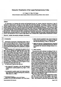
Table 2: Aggregation values for the car sales The aggregation values in Table 2 do not show the hierarchical relationship among the values. Actually, these values are derived from the base values, and there exists a hierarchical relationship. If we rearrange the values in both Table 1 and Table 2 and create a hierarchical structure as Figure 1, the relationships among all values can be revealed clearly. We can see that all values can be divided into eight groups. The number of groups is just equal to two to power of the number of dimensions that is three. Furthermore, the eight groups can be arranged into four levels according to their derivation process. The number of levels is equal to the number of dimensions plus one. The bottom group contains only base values. The second level derived from the bottom includes three groups. Each group contains aggregation values that are aggregated by removing one dimension from the bottom level. The third level is derived from the second level. It has three groups too. The values in the groups on this level are aggregated by removing one more dimension from the lower level – the second level. Finally, the top level is derived from the third level. It generates only one total aggregation value for all dimensions. Figure 1 is actually a hierarchical directed graph structure, not a tree structure. When the number of dimensions of a data cube is large, the hierarchical graph structure of the data cube will become very

complicated, which is very difficult to be represented as that in Figure 1. If we can create a visualization space that uses a tree structure to represent a data cube, the data values and relationships in the cube will be represented more clearly. Tree is a hierarchical structure. We can easily maintain the similar hierarchical structure presented in Figure 1 using a tree-based structure. To create a cube tree, the aggregation groups will be used as nodes in the tree. For those aggregation groups that are below the middle level and have more than one leaving arrowed-lines, we may need to split them into multiple nodes for the cube tree. Based on this idea, we developed a Web-based data cube visualization system. Besides maintaining the hierarchical structure, the developed system uses pies to represent nodes in the tree, and colored fans in a pie to show the aggregation values in a node. Users can also interactively control many display features to visualize a data cube in different details. ALL 941

By Model Model Sales Ford 508 GE 433

By Color Color Sales Red 233 White 369 Blue 339

By Model & Color Model Color Sales Ford Red 90 Ford White 236 Ford Blue 182 GE Red 143 GE White 133 GE Blue 157

Color Red Red Red White White White Blue Blue Blue

Model Ford Ford Ford Ford Ford Ford Ford Ford Ford GE GE GE GE GE GE GE GE GE

By Year Year Sales 2002 343 2003 314 2004 284

By Color & Year Year Sales 2002 69 2003 106 2004 58 2002 149 2003 104 2004 116 2002 125 2003 104 2004 110

Base values Year Color 2002 Red 2002 White 2002 Blue 2003 Red 2003 White 2003 Blue 2004 Red 2004 White 2004 Blue 2002 Red 2002 White 2002 Blue 2003 Red 2003 White 2003 Blue 2004 Red 2004 White 2004 Blue

By Year & Model Model Sales Ford 154 GE 189 Ford 198 GE 116 Ford 156 GE 128

Year 2002 2002 2003 2003 2004 2004

Sales 5 87 62 54 95 49 31 54 71 64 62 63 52 9 55 27 62 39

Figure 1: The hierarchical structure of a data cube

3. Web-Based Data Cube Visualization and Features Figure 2 is a snapshot of our data cube visualization system from a Web browser. The demo system is posted at http://www.cs.panam.edu/~xwang/viscube/. The system contains four panels: Control Panel, Cube Display Panel, Focused Node Panel and Group-By Panel.

Figure 2: A snapshot of the data cube visualization system 3.1 Control Panel Control panel is at the top of the user interface of the system. It consists of five control tools to allow users to load the base data values of a data cube, select view attribute, select view mode and control the view size. The first control tool is a combobox for users to select a data cube file URL. Once a file URL is selected, the file will be downloaded from the specified Web server to the visualization system. The file only contains the base data of a data cube or with parallel cubes. The first line of the file must be two numbers to specify the number of dimensions and the number of parallel date cubes. This system allows visualizing parallel data cubes. Each parallel data cube is saved as

a separate value column in the base data file. The following List 1 is a data cube source file that contains the previous Sales data cube with other two parallel data cubes: Profit and Cost. The first number 3 specifies that the data cubes have three dimensions Model, Year and Color, and the second number 3 specifies that there are three parallel data cubes Sales, Profit and Cost in this file. The second line of the file gives the names of all dimensions and parallel data cubes. These names will be used to mark the graphics objects in the visualization system later on. 3 3 Model Ford Ford Ford Ford Ford Ford Ford Ford Ford GE GE GE GE GE GE GE GE GE

Year 2002 2002 2002 2003 2003 2003 2004 2004 2004 2002 2002 2002 2003 2003 2003 2004 2004 2004

Color Red White Blue Red White Blue Red White Blue Red White Blue Red White Blue Red White Blue

Sales 5 87 62 54 95 49 31 54 71 64 62 63 52 9 55 27 62 39

Profit 40 860 610 530 940 480 300 530 700 630 610 620 510 80 540 260 610 380

Cost 25 550 420 360 670 310 200 340 450 435 410 420 330 55 350 150 400 230

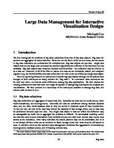
List 1: Data cube source file format The second control tool is a selection menu that allows users to select a data cube to be viewed if more than one parallel data cubes are stored in a file. Choosing different data cube name from the menu will bring the corresponding data cube to be displayed in the system. When the ALL item is selected from the menu, all parallel data cubes will be displayed in parallel in the system. This parallel data cube display mode provides a way for users to observe and compare the data relationships among different parallel data cubes. Figure 3 shows how the parallel data cubes are visualized in the system. The third control tool is another selection menu that allows users to choose the view modes. The system provides two view modes: Local and Overview. In the Local view, users can drag the tree-based data cube displayed in the Cube Display Panel, and focus on a magnified special area to see aggregation values in detail. The Overview view displays the current data cube or parallel data cubes in the Cube Display Panel completely. Both Figure 2 and Figure 3 show data cubes in the Overview view. The other two control tools are two sliders that allow users to set the Pie size and the data cube display pane size. 3.2 Cube Display Panel The Cube Display Panel is the most important panel in the system, and located at the middle left area. The size of this panel can be adjusted by dragging the vertical separate bar on the left side of the panel or the horizontal separate bar at the bottom of the panel. The Cube Display Panel uses a tree-based structure to represent the current data cube. Each node in the cube tree represents an aggregation group or a splitted aggregation group, and is displayed with a colored pie. The ALL total group in the top aggregation level of a data cube always becomes the root node of the cube tree, and is displayed at the center of the data cube tree in a gray color. The groups in other levels are displayed as colored nodes around the root node and from the center toward the outside of

the cube tree. The base values in the bottom level of a data cube are grouped into many leaf nodes that are displayed at the most outer loop of the tree. Each node is also related to a dimension of the data cube. The dimension name and the corresponding aggregation value of a node are displayed next to the colored node pie. A node pie contains several fans with different colors. The number of fans in a pie represents the cardinality of the dimension. The colors of fans in a pie represent the different values in the current dimension. The system automatically assigns an individual color to every dimension and every data value in each dimension. The size of a fan represents the percentage of a dimension value to the aggregation value in the current node. Every node in the cube tree is selectable. When the mouse cursor moves up a node, the cursor becomes a hand. This means that the current node can be selected by a single clicking. When a node is selected, a small yellow circle will be flashing on the node pie, and the corresponding node pie is magnified and displayed in the Focused Node Panel with all related aggregation values and percentage values. Moreover, the Group-By values from the root node to the current node will also dynamically be displayed with a Group-By list in the Group-By Penal. If all parallel cubes are selected from the Control Panel, the aggregation values corresponding to a node for all parallel cubes will be displayed as separate small pies on the node. Figure 3 shows that every node has three separate pies to represent the three parallel data cubes Sales, Profit and Cost.

Figure 3: A snapshot of visualization with parallel data cubes

3.3 Focused Node Panel The Focused Node Panel is used to visualize the currently selected node in detail. This panel is located on the right of the Cube Display Panel. Its size will also be changed when dragging the vertical separate bar or the horizontal separate bar. When a user selects a node in the Cube Display Panel, the selected node will be magnified and displayed in the Focused Node Panel immediately. The detailed data about the node will also be listed below the colored node pie. For a node, the colored pie visually shows the relative percentages of all individual aggregation values to the total aggregation value in the current node with colors and sizes of the fans in the pie. Sometimes, users may want to know the exact numbers about all aggregation values and their percentages to the total aggregation value in the node. Besides displaying the magnified node pie, the Focused Node Panel also lists all these numbers below the magnified node pie. The super-aggregation values for all dimensions from the root node to the current node are also listed to show the relative relationships from the root node to the current node. 3.4 Group-By Panel Many users are very familiar with the Group-By operation in SQL. The result from the Group-By operation shows aggregation values for certain attributes or dimensions clearly. Although a data cube provides all aggregation values, users may still like to read aggregation values in the Group-By list form. Our data cube visualization system provides a special panel – the Group-By Panel to display the GroupBy list dynamically. The Group-By Panel is located at the bottom of the system. Both Figure 2 and Figure 3 show this panel. As we know, a data cube generates all aggregation values that can be projected into many different Group-By lists. Which Group-By list should be displayed in the Group-By Panel at a time? Actually, when a user selects a node from the Cube Display Panel, the user usually concerns only the Group-By list from the root node to the selected node. So our system uses this principle to dynamically generate the Group-By list and displays the list in the Group-By Panel. When a node is selected, a path from the root node to the selected node is created. Based on the nodes on this path, we can determine the selected dimensions and their order, and then we can generate the Group-By list according to the selected dimensions and their order. The data items in the Group-By list are displayed with the corresponding colors that appear in the Cube Display Panel. In particular, the data item for the selected node is displayed with a gray background color. If the parallel cubes are selected, a Group-By list should include all related parallel values. Because of the space limitation in the Group-By Panel, our system does not display all parallel values in the GroupBy list at a time. Instead, we add two triangle buttons at the top-left corner of the Group-By Panel to allow users to select one parallel values for the Group-By list at a time. In Figure 3, the Group-By list only shows the Profit values. We can see there are two triangle buttons at the beginning of the Group-By Panel. By clicking the left-oriented triangle button, the Group-By list will display the Sales values. In opposite, clicking the right-oriented triangle button will cause to display the Cost values in the Group-By list.

4. Conclusions and future work In this paper, we presented our newly developed data cube visualization system. This system uses tree-based structure, simple 2D pies and colors to represent a data cube or parallel data cubes. The treebased data cubes are only displayed in a linear space. A linear space is natural and easy to be understood by users. But when dimensions and/or cardinalities of a data cube are very large, the generated cube tree will not be able to be displayed in a linear space. So at this time, the system can only be used to visualize small datasets.

Currently, this system is still under development. We will reorganize the tree structure and move the tree-based data cubes into a hyperbolic nonlinear space so that the system can be used to visualize the data cubes for large datasets. We also consider combining the hyperbolic nonlinear space with threedimensional (3D) graphics to create a 3D data cube visualization system. We believe that a 3D hyperbolic space will allow displaying a big enough data cube.

References [1] Ammoura, A., Zaiane, O., and Ji, Y., Immersed Visual Data Mining: Walking the Walk, In Proceedings of the 18th British National Conference on Databases (BNCOD'01), Oxford, UK, July 2001, pp. 202 - 218. [2] Chen, P., Hu, C., Ding, W., Lynn, H., and Yves, S., Icon-based Visualization of Large HighDimensional Datasets, In Proceedings of the 3rd IEEE International Conference on Data Mining (ICDM’03), Florida, USA, 2003, pp. 505 – 508. [3] Chen, Y., Dehne, F., Eavis, T., and Rau-Chaplin, A., Building Large ROLAP Data Cubes in Parallel, In Proceeding of the 8th International Database Engineering and Application Symposium (IDEAS’04), 2004, pp. 367 – 377. [4] Gray, J., Bosworth, A., Layman, A., and Pirahesh, H., Data Cube: A Relational Aggregation Operator Generalizing Group-By, Cross-Tab, and Sub-Totals, Microsoft Technical Report, MSR-TR-95-22, 1995. [5] Harinarayan, V., Rajaraman, A., and Ullman, J. D., Implementing Data Cubes efficiently, ACM SIGMOD Record, Vol. 25, Issue 2, 1996, pp. 205 – 216. [6] Healey, C. G., and Enns, J. T., Large Datasets at a Glance: Combining Textures and Colors in Scientific Visualization, IEEE Transactions on Visualization and Computer Graphics, Vol. 5, No. 2, April-June 1999, pp. 145 – 167. [7] Ng, R. T., Wagner, A., and Yin, Y., Iceberg-Cube Computation with PC Clusters, ACM SIGMOD Record, Vol. 30, Issue 2, June 2001, pp. 25 – 36. [8] Ross, K. A., and Srivastava, D., Fast Computation of Sparse Datacubes, In Proceedings of the 23th International Conference on Very Large Data Bases (VLDB), 1997, pp.116 – 125. [9] Smith, J. R., Li, C.-S., and Jhingran, A., A Wavelet Framework for Adapting Data Cube Views for OLAP, IEEE Transactions on Knowledge and Data Engineering, Vol. 16, No. 5, May 2004, pp.552 – 565. [10] Stolte, C., Tang, D., and Hanrahan, P., Multiscale Visualization Using Data Cubes, IEEE Transactions on Visualization and Computer Graphics, Vol. 9, No. 2, April-June 2003, pp. 176 – 187. [11] Walter, J., Ontrup, J., and Ritter, H., Interactive Visualization and Navigation in Large Data Collections Using the Hyperbolic Space, In Proceedings of the 3rd IEEE International Conference on Data Mining (ICDM’03), Florida, USA, 2003, pp. 355 – 365.