inner bound approximations of the true but unknown technologyâ and inte- grate the .... is called the directional distance function in the direction of g = (h, k).
Well-Defined Directional Distance Functions and Luenberger Productivity Indicators: Diagnosis of Infeasibilities and its Remedies Walter Briec∗ and Kristiaan Kerstens† December, 2005
Abstract A recent total factor productivity indicator presented in the literature is the Luenberger indicator based upon directional distance functions. This productivity indicator turns out to be impossible to compute under certain weak conditions. The same problems can also occur under less general productivity indicators and indexes. The purpose of this contribution is to diagnose in detail the economic conditions under which infeasibilities may occur for the case of directional distance functions and to propose some solutions that remedy the problem in an economically meaningful way. This yields a generalised productivity indicator that is always well-defined.
Keywords: Luenberger productivity indicator, infeasible directional distance function. JEL: C43, D21, D24
1
Introduction
Traditionally, total factor productivity (T F P ) growth measures in a residual way the shifts in technology, namely output growth unexplained by the input growth (Hulten (2001)). Nishimizu and Page (1982) were the first to realise that ignoring inefficiency may well bias T F P measures and they decomposed T F P growth into technical change and technical efficiency change using parametric production frontiers. Discrete time Malmquist input, output and productivity indexes based upon distance functions as general technology representations (Caves, Christensen and Diewert (1982)) have been ∗ University of Perpignan, GEREM. Correspondence: W. Briec Universit´e de Perpignan, 52 avenue de Villeneuve, F-66000 Perpignan, France. † Corresponding author: CNRS-LABORES (URA 362), IESEG, 3 rue de la Digue, F-59000 Lille, France.
1
made empirically tractable by F¨are et al. (1995). Exploiting the relation between distance functions and radial efficiency measures, they propose to compute distance functions on deterministic, nonparametric technologies – inner bound approximations of the true but unknown technology– and integrate the two-part decomposition of T F P of Nishimizu and Page (1982) into the Malmquist index. Their proposal has led to a boom in empirical studies employing the Malmquist productivity index to measure both technological and technical efficiency change (e.g., F¨are et al. (1994), among others). An important problem present in the original F¨are et al. (1995) paper is that some of the distance functions constituting the Malmquist productivity index may well be infeasible when estimated upon general technologies. These authors avoid this problem by choosing a technology with a restrictive returns to scale assumption in an effort to avoid these infeasibilities. An alternative Malmquist T F P (or Hicks-Moorsteen) index, as a ratio of Malmquist output and input indices whereby distance functions are defined evaluating hypothetical observations obtained from mixing inputs and outputs observed in two different periods, is proposed by Bjurek (1996). His proposal is at least partly motivated by the desire to avoid these infeasibilities (see page 310). Meanwhile more general primal productivity indicators have been proposed.1 For instance, Chambers and Pope (1996) and Chambers (2002) define a Luenberger productivity indicator as a difference-based index of directional distance functions. The latter functions generalise existing distance functions by accounting for both input contractions and output improvements and are dual to the profit function. As special cases, one can define input- and output-oriented versions of the Luenberger indicator, that can be interpreted as difference-based versions of the similarly oriented Malmquist productivity indices. In addition, Briec and Kerstens (2004) propose a difference-based version of the Malmquist T F P (or Hicks-Moorsteen) index. Chambers and Pope (1996: 1364) strongly argue in favour of avoiding restrictive returns to scale assumptions (e.g., constant returns to scale) that are only relevant for, e.g., a representative firm supposedly to be in long-run equilibrium. One could add that the advantage of using flexible technologies is that the resulting productivity index or indicator offers knowledge about local changes in technology. Unfortunately and hitherto unnoticed, it is possible to show that almost all of these primal productivity indices and indicators may suffer from the same problem as the Malmquist productivity index in a number of economic contexts. Since the Luenberger productivity indicator employs the most general type of distance functions (i.e., the directional distance function), this contribution focuses on defining the issue of infeasibility in this context. But, clearly most other productivity indices 1
“Indicators” denote productivity measures based on differences, while “indexes” indicate productivity measures defined as ratios (Diewert (2005)). Both approaches to index numbers are compared in Chambers (2002) and Diewert (2005), among others.
2
and indicators are also affected by the same type of problems. Of course, one option is to simply report the infeasibilities when computing productivity indices and indicators. But, unfortunately, few empirical studies explicitly report the prevalence of this infeasibility problem in, e.g., the Malmquist productivity index (see Mukherjee, Ray and Miller (2001) for an exception). Furthermore, as alluded to above, various ways of circumventing the problem have been proposed. This contribution intends to show that there is no easy solution in general. While a general solution to the problem exists under rather stringent conditions, it remains the case that in a variety of circumstances the problem of infeasibilities cannot be avoided irrespective of the estimation method used for the technology. Therefore, the purpose of this contribution is twofold. First, we diagnose in detail the economic conditions under which infeasibilities may occur for the case of directional distance functions. These are related to the choice of direction vector. Second, we propose some solutions that remedy the problem in an economically meaningful way. This analysis also permits to criticise some of the imperfect solutions suggested in this literature. To develop these arguments, this contribution is structured in the following way. Section 2 develops the basic definitions of the technology and the various distance functions. The next section states the general nature of the infeasibility problem in the definition of the directional distance function depending upon the choice of direction vector. A final section analyses the problem for the case of the Luenberger productivity indicator and provides the general solution in the case of full-dimensional non-null direction vector.
2
Technology and Distance Functions: Definitions
We first introduce the assumptions on technology and the definitions of the distance functions providing the components for computing productivity indicators. Production technology transforms inputs x = (x1 , · · · , xn ) ∈ Rn+ into outputs y = (y1 , · · · , yp ) ∈ Rp+ . For each time period t, the production possibility set T summarises the set of all feasible input and output vectors and is defined as follows: © ª T = (x, y) ∈ Rn+p + ; x can produce y .
(2.1)
Throughout the paper technology satisfies the following conventional assumptions: (T.1) (0, 0) ∈ T, (0, y) ∈ T ⇒ y = 0 i.e., no free lunch; (T.2) the set A(x) = {(u, y) ∈ T ; u 6 x} of dominating observations is bounded ∀x ∈ Rn+ , i.e., infinite outputs are not allowed with a finite input vector; (T.3) T is closed; and (T.4) ∀(x, y) ∈ T, (x, −y) 6 (u, −v) ⇒ ( u, v) ∈ T , i.e., fewer outputs can always be produced with more inputs, and inversely 3
(strong disposal of inputs and outputs). On one occasion, stronger assumptions (specifically, convexity) are needed. While these assumptions are standard, it is possible to weaken some of these maintained axioms. For instance, strong input and output disposal may be (partially) replaced by the assumption of weak disposability. Notice that in such a case the resulting technologies may lead to even more from infeasibilities of the distance functions (see below), since the production possibility set is smaller. For instance, Jaenicke (2000) notices the issue of infeasibilities for technologies with weak disposal in the output dimensions. Technology can be characterised by distance functions. To simplify the notation, we denote: z = (x, y) ∈ T. (2.2) and
g = (h , k) ∈ (−Rn+ ) × Rp+
(2.3)
which is partitioned in an input and an output direction vector h respectively k. The directional distance function involving a simultaneous input and output variation in the direction of a pre-assigned vector g is defined as: × (−Rn+ ) × Rp+ −→ R ∪ {−∞} ∪ Definition 2.1 The function DT : Rn+p + {+∞} defined by ½ sup {δ ∈ R : z + δg ∈ T } if z + δg ∈ T for some δ ∈ R DT (z; g) = −∞ otherwise is called the directional distance function in the direction of g = (h , k). Notice that distance functions are related to efficiency measures in that they measure deviations from the boundary of technology. For the purpose of studying the problem of ill-defined productivity indicators, we distinguish between the standard case where the distance is achieved and the case where there is no way to achieve the distance. This distinction is fairly standard when defining distance functions (see, e.g., Chambers (2002)). Note that when no direction is selected and a point is part of the technology (z ∈ T ), then DT (z; g) = +∞. This directional distance function (Chambers, F¨are and Grosskopf (1996)) is a special case of the shortage function (Luenberger (1992)). Note that the directional distance function is defined using a general directional vector g. However, sometimes we consider the special case: h = −x and k = y, also known as the Farrell proportional distance function (Briec (1997)).2 In the literature other direction vectors have been proposed (for instance, the translation function of Blackorby and Donaldson (1980) where h = −1n and k = 0, where 1n is the n-dimensional vector of the ones. 2
Axiomatic properties of this function are studied in Briec (1997) and Chambers, Chung and F¨are (1998).
4
See Chambers, F¨are and Grosskopf (1996) for additional choices of direction vectors. While the directional distance function is instrumental in defining the Luenberger productivity indicator, it generalises the Shephardian distance functions that are used in defining other, less general productivity indices (like the Malmquist or Hicks-Moorsteen indices). For instance, the Shephardian input distance function results by setting g = (h , 0) = (−x, 0) and calculating Di (z) = [1 − DT (z; −x, 0)]−1 . A dual formulation of the directional distance function is defined as follows: ¯ T : Rn+p Definition 2.2 The function D × (−Rn+ ) × Rp+ −→ R ∪ {−∞} + defined by ¯ T (z; g) = inf {Π(w, p) − p.y + w.x : p.k − w.h = 1} D (w,p)≥0
is called the hyper-directional distance function in the direction of g = (h , k). Chambers, Chung and F¨are (1998) prove a duality between the directional distance function and the profit function when the former function is real¯ T (z; g). Clearly, this dual version valued. In the latter case DT (z; g) = D of the directional distance function has the interpretation of a shadow profit function. While it is true that the vast majority of empirical productivity studies employ deterministic, nonparametric technologies (probably because of their advantages: (i) no problem to model multiple outputs, (ii) no need to impose a priori functional form on technology, or any restrictive assumptions regarding input remuneration), our analysis is also valid for parametric specifications of technology. An example of an empirical productivity study using both nonparametric and parametric technologies is Atkinson, Cornwell and Honerkamp (2003). The paper is phrased in terms of general technologies and does not privilege a specific estimation method.
3
Directional Distance Function: Infeasibility and its Remedy
This section analyses the precise conditions under which infeasibilities may or may not occur. This is done for general points that need not be part of technology. Notice that while the paper focuses on infeasibilities in the context of productivity indices and indicators where the problem of infeasibilities seems initially to have been noticed, it is clear that the results in this section are also useful for static contexts where out of sample methods are employed, i.e.,
5
an observation is evaluated to a technology to which it does not necessarily belong.3
3.1
Infeasible Directions
We first define the concept of an infeasible direction for the directional distance function and focus on its relationship to a general production technology. n+p let us denote: Definition 3.1 Let g ∈ (−Rn+ ) × Rp+ and for all z ∈ R+
∆(z, g) = {z + δg : δ ∈ R} the affine line generated from z in the direction of g. We say that a direction g is: a) Infeasible at z if: ∆(z, g) ∩ T = Ø; b) Interior if g ∈ (−Rn++ ) × Rp++ . We can now state the following completely general result proving that for all technologies and for an arbitrary direction vector g there exists some point z such that the direction g is infeasible at point z. The proof below is based on the characteristic of the output set P (x) that is bounded for all x ∈ Rp+ . In particular, focusing on the at least two-dimensional output case, we show that for any non-zero direction there exists an input output vector such that the direction g is infeasible. Proposition 3.2 For all technologies T satisfying T1-T4 and g ∈ (−Rn+ ) × Rp+ , if the two following conditions hold: i) the number of output dimensions is greater than or equal to 2 (p ≥ 2), ii) the output direction vector is non-zero (k 6= 0), such that the direction g is infeasible at z. then there exists some z ∈ Rn+p + All proofs are in the Appendix. To illustrate this proposition, a numerical example is provided below for a simple three dimensional production technology with two outputs. Example 3.3 Assume that n = 1 and p = 2, and let us consider the production technology: ª © T = (x, y1 , y2 ) ∈ R3+ : y1 + y2 ≤ x It is easy to check that T satisfies T 1 − T 5. Let z = (1, 0, 2), clearly z ∈ / T. Moreover, let us consider the direction g = (−1, 1, 1). The direction g is 3 One example is the measurement of gains of diversification or specialisation when considering potential candidates for mergers (see Bogetoft and Wang (2005) or F¨are, Grosskopf and Lovell (1994)). Another example is the computation of so-called super-efficiency models (e.g., Xue and Harker (2002)).
6
feasible at z if and only if the following system of linear inequalities has some solution: 1−δ ≥ 0 0+δ ≥ 0 (3.1) 2+δ ≥ 0 2 + 2δ ≤ 1 − δ Clearly, the system (3.1) has no solution and thereby DT (z; g) = −∞. Following Proposition 3.2, for a given technology with a number of outputs p ≥ 2 and a given direction vector with non-null output direction, there always exists an input output vector such that the directional distance function takes the value −∞. Corollary 3.4 For all production technologies T satisfying T1-T4 where p ≥ n+p 2 and all g ∈ Rn+p such that D(z; g) = −∞. + , there exists z ∈ R+ This implies that one can always find a direction vector (with non-null output direction) which is infeasible for a given point z. Corollary 3.5 For all production technologies T satisfying T1-T4 where p ≥ such that D(z; g) = −∞. and z ∈ Rn+p 2, there exists g ∈ Rn+p + + Thus, this perfectly general result demonstrates that even the Luenberger productivity indicator, that employs the most general of distance functions, cannot avoid infeasibilities. Furthermore, these results can serve to illustrate that some claims in the literature regarding the origin of the infeasibility problem are simply wrong. For instance, the output-oriented Malmquist productivity index can well be infeasible irrespective of the maintained returns to scale assumption on technology. As another example, Jaenicke (2000: 257-258) suggests that imposing strong instead of weak output disposal on technology is sufficient to guarantee feasibility for a distance function with non-null output direction vector when constructing an output-oriented Malmquist index. This claim is erroneous, since even with the stronger assumption of strong output disposal maintained in this contribution it is impossible to rule out infeasibilities. However, the above results are no longer valid when the output set in onedimensional and the direction vector is semi-positive in inputs and positive in the single output, as it is stated in the next result. Lemma 3.6 Let T be a production technology satisfying T1-T4. If the output set is one-dimensional (p = 1) and if g ∈ (−Rn+ )×R++ , then for all z ∈ Rn+1 + , the direction g is feasible at z.
7
3.2
Infeasible Directions When the Output Direction Vector is Null
Now, we focus on the case where the output direction is null. Here, the eventual infeasibilities depend on the precise choice of the input direction. We can formulate a first general result as follows: Proposition 3.7 Let T be a production technology satisfying T 1 − T 4. Let y ∈ Rp+ and assume that L(y) 6= Ø. Assume there exist i0 ∈ {1, · · · , n} and αi0 ≥ 0 such that for all u ∈ L(y), ui0 > αi0 . If g = (h, 0) is a direction such that hi0 = 0, then there exists some x ∈ Rn+ such that the direction g is infeasible at point z = (x, y) for all y ∈ Rp+ . Thus, whenever output direction is null, at least one input dimension is essential (i.e., there is a minimal level needed of this input to produce some outputs), and the input direction vector is not of full dimension in the essential input(s), there is always a point such that it is infeasible for a general technology. A simple numerical example based on a Leontief technology is provided below showing that this type of infeasibility may well appear in a traditional parametric technology. Example 3.8 Assume that T = {(x1 , x2 , y) ∈ R3+ : y ≤ min{x1 , x2 }}. If g = (−1, 0, 0), then the direction g is infeasible at point (1, 12 , 1). The next example focus on the more general Cobb-Douglas technology. Example 3.9 Assume that T = {(x1 , x2 , y) ∈ R3+ : y ≤ xθ11 xθ22 }, where θ1 , θ2 > 0. If g = (−1, 0, 0), then the direction g is infeasible at point (0, 1, 1). In conclusion of both examples, it is clear that traditional parametric technology specifications are not immune to the infeasibility problem. Next, we show that when the output correspondence is bounded4 , then for all input-oriented directions there exists an infeasible direction at some point in Rn+p + . Furthermore, if an output vector is attainable from an input vector and the direction vector is interior in the inputs, then the directional distance function is feasible. Proposition 3.10 Let T be a production technology satisfying T 1 − T 4. We have the following properties: a) If P is a bounded correspondence, then for all directions g = (h, 0), there exists some z ∈ Rn+p such that g = (h, 0) is an infeasible direction at z. + b) Assume that y ∈ P (Rn+ ) and suppose that the input set L(y) has a nonempty interior in Rn+ . If h ∈ −R++ , then the input interior direction g = (h, 0) is feasible at z = (x, y). We say that the output correspondence is bounded if there exists a compact K ⊂ Rp+ such that P (x) ⊂ K for all x ∈ Rn+ . 4
8
To illustrate the a) part of this proposition, we cite a few empirical studies explicitly reporting the prevalence of this infeasibility problem in the case of the input-oriented Malmquist index. Glass and McKillop (2000) mention for their sample of 84 UK building societies that 5, 6 and 6 observations (about 7%) encounter infeasibilities when comparing their distances to technologies situated in different time periods. Mukherjee, Ray and Miller (2001) report between 1% and 3.5% infeasibilities on a larger sample of 201 US commercial banks over a longer number of years (see their Tables 4-6). The following corollary is immediate: Corollary 3.11 Let T be a production technology satisfying T 1 − T 4. Moreover, assume that T has a nonempty interior, p = 1 and constant returns to scale hold. For all y ∈ R+ if h ∈ −Rn++ , then the input interior direction g = (h, 0) is feasible at z = (x, y). This corollary explains that in the single output case imposing constant returns to scale and a full dimensional input direction vector are sufficient conditions for feasibility. In the literature on the Malmquist productivity index, the impression is given that the infeasibility issue can be solved by simply imposing constant returns to scale on a non-parametric technology (see, e.g., F¨are, Grosskopf and Lovell (1994)). However, the above propositions clearly demonstrate that the occurrence of infeasibilities in, for instance, the case of the input-oriented Malmquist index is not linked to a returns to scale hypothesis imposed on technology, but that it depends on the output direction vector being null and the input direction vector not being of full dimension. Furthermore, constant returns to scale in itself is never a sufficient condition to guarantee feasibility. Thus, both the use of parametric and non-parametric technologies can generate infeasibilities when computing discrete time productivity indexes when the output direction vector is null and the input direction vector is not of full dimension.
3.3
Duality and Feasibility
One of the key results so far, proven in Proposition 3.2, is that if k 6= 0 then such that the direction g is infeasible at z. Therefore, there is some z ∈ Rn+p + n+p it is obvious that if g ∈ (−Rn++ ) × Rp++ , then there is some z ∈ R+ such that DT (z; g) = −∞. In this subsection we show, perhaps surprisingly, that this results does not hold true for the dual formulation of the directional distance function. To show this, we introduce the free disposal cone that is defined as: K = Rn+ × (−Rp+ )
(3.2)
This cone is related to the free disposal assumption because T4 can be equivalently written as (T + K) ∩ Rn+p = T . Throughout this subsection this free + disposal cone plays a crucial role. 9
The next main result establishes that if the line ∆(z, g) meets the addition of the technology and the free disposal cone T + K, then the dual directional distance function is well-defined. Proposition 3.12 Let T be a production technology satisfying T1-T5. For all z ∈ Rn+p + , if ∆(z, g) ∩ (T + K) 6= Ø, then: ¯ T (z; g) > −∞, D and:
¯ T (z; g) = max{δ : z + δg ∈ T + K}. D
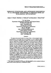
Moreover, there exist (¯ x, y¯) ∈ Rn+p and (w, ¯ p¯) ∈ Rn+p with p¯.k − w.h ¯ =1 + + such that: ¯ T (z; g) = p¯.¯ D y − w.¯ ¯ x − p¯.y + w.x. ¯ This has an immediate consequence: if all components of the direction vector are non-zero, then the dual directional distance function is well-defined. Otherwise, the dual directional distance function may well not solve the infeasibility problem. Corollary 3.13 Let T be a production technology satisfying T1-T5. Let g ∈ n+p , we have: (−Rn++ ) × Rp++ be an interior direction. For all z ∈ R+ ¯ T (z; g) > −∞. D Another corollary points out the difference between primal and dual directional distance functions for some infeasible directions. Corollary 3.14 Let T be a production technology satisfying T1-T-5. For all z ∈ Rn+p + , if ∆(z, g) ∩ T = Ø and ∆(z, g) ∩ (T + K) 6= Ø, then: ¯ T (z; g) > DT (z; g) = −∞. D This last result is illustrated in Figure 1. In Figure 1, we suppose that ¯ T (z; g) = such that D g = (0, k). Therefore, for all price vectors (w, ¯ p¯) ∈ Rn+p + Π(w, ¯ p¯) − p¯.y + w.x ¯ with p¯.k − w.h ¯ = 1, we have Π(w, ¯ p¯) − p¯.y + w.x ¯ = p¯.(y + γ(z; g)k) − w.(x ¯ + γ(z; g)h) − p¯.y + w.x ¯ = p.(y + γ(z; g)k) − p¯.y = R(¯ p, x)− p¯.y > 0. Thus, there exist points and direction vectors for which the hyper-directional distance function may well be feasible, while the directional distance function is infeasible.
10
y2
6
p.y
y
R(p, x)
7
k P (x)
- y1
0 P (x) − Rp+
¯ T (z; g) > −∞. Figure 1 A case where DT (z; g) = −∞ and D
This same result is also illustrated by taking up again the earlier Example 3.3 and showing that its dual directional distance function is feasible. Example 3.15 Let us consider Example 3.3 where for n = 1 ªand p = 2, © the production technology is T = (x, y1 , y2 ) ∈ R3+ : y1 + y2 ≤ x . We have shown that the direction g = (−1, 1, 1) is not feasible at point z = (1, 0, 2) and thereby DT (z; g) = −∞. However, we have shown in Proposition 3.12 ¯ T (z; g) = sup{δ : (1, 0, 2) + that the dual directional distance function is D δ(−1, 1, 1) ∈ T + K}. Let us determine a maximization program to compute this dual directional distance function. Since the output dimension is not constrained in T + K, we have: © ª T + K = (x, y1 , y2 ) ∈ R+ × R2 : y1 + y2 ≤ x Therefore, the constraints 0 + δ ≥ 0 and 2 + δ ≥ 0 in system 3.1 should be suppressed in the maximization program to compute the dual directional distance function: max δ 1−δ ≥ 0 (3.3) 2 + 2δ ≤ 1 − δ ¯ T (z; g) = −1/3 > −∞ = DT (z; g). We obtain D To complete the main result above we establish that if the condition ∆(z, g) ∩ (T + K) 6= Ø does not hold, then the dual directional distance ¯ T (z; g) = −∞). function is infeasible (D Proposition 3.16 Let T be a production technology satisfying T1-T5. For all z ∈ Rn+p + , if ∆(z, g) ∩ (T + K) = Ø, then: ¯ T (z; g) = −∞. D 11
To conclude this discussion, we establish a final result indicating that the feasibility of the dual directional distance function is a necessary and sufficient condition to conclude that the intersection of a line with the technology extended by the free disposal cone is non-empty. Theorem 3.17 Let T be a production technology satisfying T1-T5. For all z ∈ Rn+p + , ¯ T (z; g) = −∞. ∆(z, g) ∩ (T + K) = Ø ⇐⇒ D Example 3.18 Recently, Chambers, F¨are and Grosskopf (1996) provide programs to compute the Luenberger productivity indicator (see below) using non-parametric technologies (see Varian (1984) and Banker and Maindiratta (1988)). These programs involve possible infeasibilities. Let J = {1, · · · , J} and consider the set of activities Ak = {z j : j ∈ J }. Suppose that (0, 0) ∈ A and xj = 0 =⇒ y j = 0 (to obey axioms T1-T5). The non-parametric estimate Tˆ of the unknown technology based on the observed set of data A is: © ª n+p j j Tˆ = z ∈ Rn+p , + : ∀(w, p) ∈ R+ , ∃j ∈ J with p.y − w.x ≤ p.y − w.x (3.4) which can equivalently be rewritten as: ¾ ½ n+p n+p j j Tˆ = z ∈ R+ : ∀(w, p) ∈ R+ , r.y − w.x ≤ max{p.y − w.x } . (3.5) j∈J
From Varian (1984) and Banker and Maindiratta (1988), the primal formulation of this non-parametric technology can be written: ª © m (3.6) Tˆ = z ∈ Rn+p + : x ≥ Xθ, y ≤ Y θ, 1 .θ = 1, θ ≥ 0 where X is a n × m input matrix whose j-th row is xj , and Y is a p × m output matrix whose j-th row is y j . 1m is the m-dimensional unit vector. ¯ ˆ (z; g) = sup{δ ∈ R : z + δg ∈ Tˆ + K}, Now, since we have established that D T we immediately have: ¯ ˆ (z; g) = sup {δ ∈ R : x + δh ≥ Xθ, y + δk ≤ Y θ, 1m .θ = 1, θ ≥ 0} . D T (3.7) This program proposed by Chambers, F¨are and Grosskopf (1996) does not calculate the directional distance function. Indeed, to calculate this function one should impose the condition y + δk ≥ 0, because (x, y) may not be in Tˆ and in such a case DTˆ (z; g) < 0. Consequently, the correct formulation for computing the the directional distance function is: DTˆ (z; g) = sup {δ ∈ R : x + δh ≥ Xθ, y + δk ≤ Y θ, y + δk ≥ 0, 1m .θ = 1, θ ≥ 0} . (3.8) This proves that the program in (3.7) may well generate erroneous results when (x, y) ∈ / Tˆ. 12
3.4
Existence of Feasible Directions
This subsection sets to determine the conditions for the existence of a feasible direction g˜(z) at each point z in the non-negative Euclidean orthant. It turns out that the required necessary and sufficient conditions are very restrictive. For convenience, we use the following decomposition of the direction vector ˜ ˜ g˜(z) = (h(z), k(z)). More specifically, suppose that the direction vector is given by some function g˜ : Rn+p −→ (−Rn+ ) × Rn+ termed the direction + function. This direction function is defined as: ˜ ˜ g˜(z) = (h(z), k(z)).
(3.9)
Proposition 3.19 Assume that p ≥ 2. Then, the two following conditions are equivalent: n+p i) For all production technologies satisfying T1-T4 and all z ∈ R+ , ∆(z, g˜(z))∩ T 6= Ø ˜ ii) g˜ has the form g˜(z) = (h(z), cy) where c ∈ R++ . Thus, when the direction vector is interior and strictly proportional in all output dimensions in the technology (and p ≥ 2), then the directional distance function is always feasible. The following corollary is an immediate consequence. Corollary 3.20 For all production technology satisfying T1-T4 and all z ∈ ˜ ˜(z) = (h(z), cy) where c ∈ R++ , Rn+p + , if the direction function has the form g then DT (z; g˜(z)) > −∞. The above conditions underscore the importance of imposing minimal restrictions on the output direction to guarantee feasibility. The next result establishes necessary and sufficient conditions in the case of an input-oriented direction vector. It turns out that if the output direction vector equals zero and an output vector is attainable from an input vector, then a necessary and sufficient condition for the directional distance function to be feasible is that the direction vector is input interior for all production vectors z. −→ (−Rn+ ) × {0}p is a direction Proposition 3.21 Suppose that g˜ : Rn+p + n+p function. Let (x, y) ∈ R+ and suppose that y ∈ P (Rn+ ). The two following conditions are equivalent: i) For all production technologies satisfying T1-T4 and all z ∈ Rn+p ˜(z))∩ + , ∆(z, g T 6= Ø n ˜ ˜ n+p ii) g˜ has the form g˜(z) = (h(z), 0) where h(R + ) ⊂ −R++ . This excludes all sub-vector orientations in the inputs when the output direction vector is null. Ouellette and Vierstraete (2004) are an example of a study reporting infeasibilities (in particular, 1 out of 15 observations) for a sub-vector input-oriented Malmquist productivity index. 13
4
Luenberger Productivity Indicator: Diagnosing its Infeasibility
4.1
Luenberger Productivity Indicator: Definition
In the remainder of this contribution the production possibility set at time period t is denoted as T t . Thus, the set of all feasible input and output vectors is formalized as follows: © ª t t T t = (xt , y t ) ∈ Rn+p . (4.1) + ; x can produce y where xt and y t represent respectively the input and output vectors at time t. Now it is necessary to focus on a slightly more general formulation of the directional distance function. Suppose that the direction vector is given by some direction function g˜ : Rn+p −→ (−Rn+ ) × Rn+ . Hence, the directional + distance function is DT (z; g˜(z)). Therefore, if g˜(z) = g is independent of z, one retrieves the usual formulation of the the directional distance function due to Chambers, Chung and F¨are (1998). Moreover, to simplify notation, denote: ¯ t (z t ; g˜(z t )) = D ¯ T t (z t ; g˜(z t )). Dt (z t ; g˜(z t )) = DT t (z t ; g˜(z t )) and D
(4.2)
Following Chambers (2002), the difference-based Luenberger productivity indicator L(z t , z t+1 ; g˜) in the general case of a direction function is defined as follows: L(z t , z t+1 ; g˜) =
1 2
t+1 t+1 [(Dt (z t ; g˜(z t )) ¡ − Dt (zt ; tg˜(z ))) t+1 ¢¤ + Dt+1 (z ; g˜(z )) − Dt+1 (z ; g˜(z t+1 )) . (4.3) When g˜(x, y) = (−x, y), then one obtains a proportional Luenberger indicator, as mentioned in Chambers, F¨are and Grosskopf (1996). To avoid an arbitrary choice of base years, an arithmetic mean of a difference-based Luenberger productivity indicator in base year t (first difference) and t+1 (second difference) is taken. Productivity growth (decline) is indicated by positive (negative) values. Notice that general definitions of the directional distance functions introduced above imply that the Luenberger productivity indicator may well not be real-valued. Empirical studies reporting this phenomenon, however, are not known to us. It is equally possible to define input- and output-oriented versions of this Luenberger productivity indicator based on the input respectively the output directional distance functions. Evidently, the same infeasibilities would reappear.
4.2
Undefined Luenberger Productivity Indicator
The next example shows that there exist technologies obeying axioms T 1−T 4 for which there exist g, z t and z t+1 such that the direction g is infeasible both 14
at z t with respect to T t+1 and at z t+1 with respect to T t . Thus, the mixedperiod directional distance functions cannot be computed. Example 4.1 Assume that T t = {(x, y1 , y2 ) ∈ R3 : max{ y81 , y2 } ≤ x} and T t+1 = {(x, y1 , y2 ) ∈ R3 : max{y1 , y82 } ≤ x}. Clearly, z t = (1, 8, 1) ∈ T t and z t+1 = (1, 1, 8) ∈ T t+1 . Suppose that the direction function is constant. By taking g = (0, 1, 1) it is easy to see that g is not feasible at z t with respect to T t+1 and in the same way it is not feasible at z t+1 with respect to T t . As an immediate consequence there exist technologies T t and T t+1 such that the Luenberger productivity indicator is not defined when the number of output dimensions is greater than 1. This means that the Luenberger productivity indicator may not take its values in [−∞, +∞] and remains undefined. Proposition 4.2 Suppose that the direction function g˜ is constant and p ≥ 2. There exists a pair of technologies T t and T t+1 satisfying T1-T4 that respectively contain z t 6= (0, 0) and z t+1 6= (0, 0), such that L(z t , z t+1 ; g) is not defined.
4.3
Well-Defined Luenberger Productivity Indicators
The next result establishes necessary and sufficient conditions to make the Luenberger productivity indicator computable for all technologies. In particular, it shows that when the number of output dimensions is greater than 1, then the output direction should be proportional to the output vector. Clearly, this condition is a straightforward consequence of Proposition 3.19 above. Proposition 4.3 Assume that p ≥ 2. The two following conditions are equivalent: i) For all pairs of technologies T t and T t+1 that respectively contain z t 6= (0, 0) and z t+1 6= (0, 0), L(z t , z t+1 ; g) is defined. ˜ ii) g˜ has the form g˜(z) = (h(z), cy) where c ∈ R++ . This result is a direct consequence of Proposition 3.19 and seems to indicate that the choice of a proportional output direction vector seems highly desirable. This could be interpreted as an argument in favour of the proportional distance function, whereby the direction vector equals the evaluated observation (see Chambers, F¨are and Grosskopf (1996) for a discussion of various choices of direction vector). It has been shown before that there exists some cases where, in spite of the infeasibility of a direction, the dual directional distance function is well-defined. For that reason, it is possible to define a dual Luenberger productivity indicator that is well-defined, at least for interior directions (i.e., directions being non-null in all dimensions). Following Balk (1998), the hyper-Luenberger productivity indicator is defined by: 15
¯ t , z t+1 ; g˜) = L(z
1 2
£¡
¢ ¯ (z t ; g˜(z t )) − D ¯ (z t+1 ; g˜(z t+1 )) D t t ¡ ¢¤ ¯ (z t ; g˜(z t )) − D ¯ (z t+1 ; g˜(z t+1 )) . + D t+1 t+1
(4.4)
Since from Corollary 3.13 the hyper-directional distance function is welldefined for interior directions, the hyper-Luenberger productivity indicator is also well-defined under the same conditions. Of course, since duality is involved in the construction of the hyper-directional distance function, one must impose convexity of technology in the next result. Proposition 4.4 Suppose that g˜ : Rn+p −→ (−Rn++ ) × Rp++ , i.e., the direc+ tion function is interior. For all pairs of technologies T t and T t+1 satisfying ¯ t , z t+1 ) is T1-T5 that respectively contain z t 6= (0, 0) and z t+1 6= (0, 0), L(z well-defined. Thus, only in the case of interior directions, the dual Luenberger productivity indicator is well-defined. Otherwise, there is no guarantee for it being well-defined.5 Furthermore, it is clear that no general solution exists in the case of non-convex technologies.
4.4
Infeasibility and Luenberger-Hicks-Moorsteen Productivity Indicator
Briec and Kerstens (2004) define the Luenberger-Hicks-Moorsteen T F P indicator, a difference-based version of the Hicks-Moorsteen index. A LuenbergerHicks-Moorsteen indicator with base period t is defined as the difference between a Luenberger Output Quantity indicator and a Luenberger Input Quantity indicator: LHMt (z t , z t+1 ) = LOt (z t ,z t+1 , g) − LIt (z t , z t+1 ,g)
(4.5)
LOt (z t , z t+1 ) = Dt (xt ,y t+1 ; 0, k(z t+1 )) − Dt (z t ; 0, k(z t ))
(4.6)
LIt (z t , z t+1 ) = Dt (xt+1 ,y t ; h(z t+1 ), 0) − Dt (z t ; h(z t ), 0).
(4.7)
where and Remark that a slightly more general definition of direction vector of the directional distance function has been employed. In particular, if h(x, y) = x 5
In fact, also productivity indices and indicators based upon economic value functions (e.g., cost function) may well suffer from the same problems unless they have the equivalent of interior directions (e.g., long-run cost functions rather than short-run cost functions). Examples could be the decomposition of the Fisher ideal productivity index presented in Ray and Mukherjee (1996: pages 1672-1674), or the Bennet indicator analysed by GrifellTatj´e and Lovell (1999). We do not explicitly treat these cases because it would lead us too far, but simply note that our basic diagnosis and solutions probably remain valid.
16
and k(x, y) = y for all (x, y) ∈ Rn+p + , then we retrieve the formulation due to Briec and Kerstens (2004). Also a base period t + 1 Luenberger T F P indicator can be similarly defined as follows: LHMt+1 (z t , z t+1 ) = LOt+1 (z t , z t+1 ) − LIt+1 (z t , z t+1 )
(4.8)
where LOt+1 (z t , z t+1 ) = Dt+1 (z t+1 ; 0, k(z t+1 )) − Dt+1 (xt+1 ,y t ; 0, k(z t ))
(4.9)
LIt+1 (z t , z t+1 ) = Dt+1 (z t+1 ; h(z t+1 ), 0) − Dt+1 (xt ,y t+1 ; h(z t ), 0).
(4.10)
and
Remark again that this definition of the direction vector is more general. An arithmetic mean of these two base periods Luenberger T F P indicators is: LHMt,t+1 (z t , z t+1 ) =
¤ 1£ LHMt (z t , z t+1 ) + LHMt+1 (z t , z t+1 ) . 2
(4.11)
These Luenberger output quantity and Luenberger input quantity indicators are generalisations of the Malmquist output and input quantity indices defined in Chambers, F¨are and Grosskopf (1994). When the Luenberger T F P indicator is larger (smaller) than zero, it indicates productivity gain (loss). Crucial for our purpose is that this type of T F P indicator does not encounter any problems of infeasibilities under some weak conditions. Now we first establish a result proving that the Luenberger T F P index may not be defined for some pairs of technologies when one of the input dimensions of the direction vector is zero. The following example is helpful. Example 4.5 Assume that T t = {(x1 , x2 , y1 , y2 ) ∈ R4+ : max{ y81 , y2 } ≤ min{ x81 , x2 }} and T t+1 = {(x1 , x2 , y1 , y2 ) ∈ R4+ : max{y1 , y82 } ≤ min{x1 , x82 }}. Clearly, z t = (8, 1, 8, 1) ∈ T t and z t+1 = (1, 8, 1, 8) ∈ T t+1 . Suppose that the direction function is constant. By taking g = (0, −1, 1, 1), it is easy to see that h = (0, −1) is not feasible at (xt , y t+1 ) = (8, 1, 1, 8) with respect to T t+1 . Moreover, k = (1, 1) is not feasible at (xt+1 , y t ) = (1, 8, 8, 1) with respect to T t. Proposition 4.6 Suppose that the direction function g is constant and p ≥ 2. There exist a pair of technologies T t and T t+1 which respectively contain z t 6= (0, 0) and z t+1 6= (0, 0), such that LHM (z t , z t+1 ; g) is not defined. The next result establishes necessary and sufficient conditions to make the Luenberger T F P indicator computable for all technologies. These conditions are only slightly more restrictive than those established for the Luenberger 17
productivity indicator. Again if the output dimension is greater than 1, then the output direction should be proportional to the output vector. However, since input orientations are also involved in the construction of the Luenberger T F P indicator, another restriction is needed to make the Luenberger T F P indicator feasible, namely that all input component of the direction vector should be positive. Clearly, this condition is a straightforward consequence of Proposition 3.21. Proposition 4.7 Assume that p ≥ 2. The two following conditions are equivalent: i) For all pair of technologies T t and T t+1 which respectively contain z t 6= (0, 0), and z t+1 6= (0, 0), LHM (z t , z t+1 ; g) is defined. n+p ii) g has the form g(z) = (h(z), cy) where c ∈ R++ and h(R+ ) ⊂ −Rn++ . When some of the input dimensions are zero, the only alternative way to guarantee feasibility is to redefine the Luenberger T F P indicator in such a way that these dimensions are from the adjacent time period. As previously indicated, the Hicks-Moorsteen index is based upon a ratio of combinations of output-oriented Shephardian distance functions with null input direction vectors and input-oriented distance functions with null output direction vectors. This ratio-based version of the above Luenberger T F P indicator is feasible under similar conditions.
5
Conclusions
This paper has verified in detail under which conditions the directional distance function, the most general distance function introduced in the literature so far, may not achieve its distance in the general case where a point need not be part of technology and where the direction vector can take any value. This problem was studied because of its potential importance for the Luenberger productivity indicator, the most general among the recent productivity indices and indicators based upon primal information. In section 2 we demonstrated a perfectly general result that in the case of more than two output dimensions and non-null output direction vector, the directional distance function may be infeasible. In addition to a series of more specific infeasibility results, it has been demonstrated that the hyper-directional distance function, the dual version of the standard directional distance function, is always feasible for interior directions. Turning to the implications of these results for maintaining feasibility at the level of the Luenberger productivity indicator, it has been shown that this can only be guaranteed for non-null points with direction vectors in some sense proportional to these points. The dual Luenberger productivity indicator is well-defined for interior directions only, but this requires the additional axiom of convexity. 18
Apart from reporting any eventual infeasibilities (which seems to be rarely done), this contribution indicates under which circumstances one can expect infeasibilities to occur and when these can be avoided. Further research could eventually verify the possibility to restrict the choices open for the direction vectors in order to limit the incidence of infeasibilities. The current results can be partly interpreted as providing support for the proportional directional distance function, whereby the direction vector equals the evaluated observation.
References Atkinson, S.E., C. Cornwell, O. Honerkamp (2003) Measuring and Decomposing Productivity Change: Stochastic Distance Function Estimation Versus Data Envelopment Analysis, Journal of Business and Economic Statistics, 21(2), 284-294. Balk, B.M. (1998) Industrial Price, Quantity, and Productivity Indices: The Micro-Economic Theory and an Application, Boston, Kluwer. Banker, R.D., A. Maindiratta (1988) Nonparametric Analysis of Technical and Allocative Efficiencies in Production, Econometrica, 56(6), 1315-1332. Bjurek, H. (1996) The Malmquist Total Factor Productivity Index, Scandinavian Journal of Economics, 98(2), 303-313. Blackorby, C., D. Donaldson (1980) A Theoretical Treatment of Indices of Absolute Inequality, International Economic Review, 21(1), 107136. Bogetoft, P., D. Wang (2005) Estimating the Potential Gains from Mergers, Journal of Productivity Analysis, 23(2), 145-171. Briec, W. (1997) A Graph Type Extension of Farrell Technical Efficiency Measure, Journal of Productivity Analysis, 8(1), 95-110. Briec, W., K. Kerstens (2004) A Luenberger-Hicks-Moorsteen Productivity Indicator: Its Relation to the Hicks-Moorsteen Productivity Index and the Luenberger Productivity Indicator, Economic Theory, 23(4), 925 939. Caves, D.W., L.R. Christensen, W.E. Diewert (1982) The Economic Theory of Index Numbers and the Measurement of Input, Output, and Productivity, Econometrica, 50(6), 1393-1414.
19
Chambers, R.G. (2002) Exact Nonradial Input, Output, and Productivity Measurement, Economic Theory, 20(4), 751-765. Chambers, R.G., Y. Chung, R. F¨are (1998) Profit, Directional Distance Functions, and Nerlovian Efficiency, Journal of Optimization Theory and Applications, 98(2), 351 364. Chambers, R.G., R. F¨are, S. Grosskopf (1994) Efficiency, Quantity Indexes, and Productivity Indexes: A Synthesis, Bulletin of Economic Research, 46(1), 1-21. Chambers, R.G., R. F¨are, S. Grosskopf (1996) Productivity Growth in APEC Countries, Pacific Economic Review, 1(3), 181-190. Chambers, R.G., R.D. Pope (1996) Aggregate Productivity Measures, American Journal of Agricultural Economics, 78(5), 1360-1365. Diewert, W.E. (2005) Index Number Theory Using Differences Rather than Ratios, American Journal of Economics and Sociology, 64(1), 347-395. F¨are, R., E. Grifell-Tatj´e, S. Grosskopf, C.A.K. Lovell (1997) Biased Technical Change and the Malmquist Productivity Index, Scandinavian Journal of Economics, 99(1), 119-127. F¨are, R., S. Grosskopf, B. Lindgren, P. Roos (1995) Productivity Developments in Swedish Hospitals: A Malmquist Output Index Approach, in: A. Charnes, W.W. Cooper, A.Y. Lewin, and L. M. Seiford (eds) Data Envelopment Analysis: Theory, Methodology and Applications. Kluwer, Boston, 253-272. F¨are, R., S. Grosskopf, C.A.K. Lovell (1994) Production Frontiers, Cambridge, Cambridge University Press. F¨are, R., S. Grosskopf, M. Norris, Z. Zhang (1994) Productivity Growth, Technical Progress, and Efficiency Change in Industrialized Countries, American Economic Review, 84(1), 66-83. Glass, J.C., D.G. McKillop (2000) A Post Deregulation Analysis of the Sources of Productivity Growth in UK Building Societies, Manchester School, 68(3), 360-385. Grifell-Tatj, E., C.A.K. Lovell (1999) Profits and Productivity, Management Science, 45(9), 1177-1193. Hulten, C.R. (2001) Total Factor Productivity: A Short Biography, in: C.R. 20
Hulten, E.R. Dean, M.J. Harper (eds) New Developments in Productivity Analysis, Chicago, University of Chicago Press, 1-47. Jaenicke, E.C. (2000) Testing for Intermediate Outputs in Dynamic DEA Models: Accounting for Soil Capital in Rotational Crop Production and Productivity Measures, Journal of Productivity Analysis, 14(3), 247-266. Mukherjee, K., S.C. Ray, S.M. Miller (2001) Productivity Growth in Large US Commercial Banks: The Initial Post-Deregulation Experience, Journal of Banking and Finance, 25(5), 913-939. Nishimizu, M., J. Page (1982) Total Factor Productivity Growth, Technological Progress and Technical Efficiency Change: Dimensions of Productivity Change in Yugoslavia, 1965-78, Economic Journal, 92(368), 920-936. Ouellette, P., V. Vierstraete (2004) Technological Change and Efficiency in the Presence of Quasi-Fixed Inputs: A DEA Application to the Hospital Sector, European Journal of Operational Research, 154(3), 755-763. Ray, S.C., K. Mukherjee (1996) Decompositions of the Fisher Ideal Index of Productivity: A Non-Parametric Dual Analysis of US Airlines Data, Economic Journal, 106(439), 1659-1678. Varian, H. (1984) The Nonparametric Approach to Production Analysis, Econometrica, 52(3), 579-597. Xue, M., P.T. Harker (2002) Ranking DMUs with Infeasible Super-Efficiency DEA Models, Management Science, 48(5), 705-710.
Appendix Proof of Proposition 3.2: We first consider the case where there is some j ∈ {1, · · · , p} such that kj = 0. Since p ≥ 2, this does not contradict kj 6= 0. Now, consider some x ∈ Rn+ and let P (x) = {y ∈ Rp+ : x can produce y}. Since P (x) is compact, there exists some y¯ such that P (x) ⊂ {v ∈ Rp+ : y ≤ y¯}. Let y ∈ Rp+ such that yj > y¯j . Then, for all δ ∈ R, yj + δkj = yj > y¯j . Thus, y + δk ∈ / {v ∈ Rp+ : y ≤ y¯}. Thus, y + δk ∈ / P (x). Consequently, n+p (x, y) + δg ∈ / T . Since z = (x, y) ∈ R+ , we deduce that g is infeasible at z. Assume now that for all j ∈ {1, · · · , p}, kj > 0. Since P (x) is compact, there is j ∈ {1, · · · , p} and some y ∈ Rp+ such that y ∈ {v ∈ Rp : vj = 0} and y ∈ / P (x). For all δ ≥ 0, y + δk ∈ P (x) =⇒ y ∈ P (x) (from the strong disposal assumption). This is a contradiction, thus for all δ ≥ 0, we have 21
y + δk ∈ / P (x). Moreover, since yj = 0, δ < 0 =⇒ yj + δk ∈ / Rp+ =⇒ y + δk ∈ / P (x). Thus, we deduce that (x, y) + δg ∈ / T , for all δ ∈ R. This ends the proof. 2 Proof of Lemma 3.6: Assume that z ∈ / T . Let δ¯ = −y . We have k n n ¯ ¯ ¯ z + δg = (x+ δh, 0). Since h ∈ −R+ , we deduce that z + δg ∈ R+ ×{0}. Since ¯ ∈ T. 2 (0, 0) ∈ T , we deduce from the strong disposal assumption that z + δg Proof of Proposition 3.7: We just consider the vector x ∈ Rn+ defined by ½ 1 if i 6= i0 xi0 = αi0 if i = i0 2 for i = 1 · · · n. Now, let h ∈ −Rn+ such that hi0 = 0. Now, it is clear that α for all δ ∈ R, xi0 + δhi0 = 2i0 ≤ αi0 . But, since for all u ∈ L(y), ui0 > αi0 , we deduce that x + δh ∈ / L(y). Consequently, for all vector k ∈ Rp+ , and all p y ∈ R+ , (x, y) + δg ∈ / T , this ends the proof. 2 Proof of Proposition 3.10: a) If P (x) is a bounded set, then there exists / P (x). Now for all δ ∈ R, we have (x, y) + δ(h, 0) ∈ /T y ∈ Rp+ such that y ∈ and this ends the proof. b) Since L(y) has a nonempty interior, there is some u ∈ L(y) ∩ Rn++ . Moreover, since h ∈ Rn++ , there is some δ¯ ∈ R such ¯ ≥ u. Since the free disposal assumption holds, we deduce that that x + δh ¯ x + δh ∈ L(y). This ends the proof. 2 Proof of Corollary 3.11: Since T has a nonempty interior, then L(y) has also a nonempty interior in Rn+ . However, since p = 1 for all y ∈ R+ , L(y) 6= Ø and this ends the proof. 2 Proof of Proposition 3.12: Let us denote γ(z; g) = sup{δ : z + δg ∈ T + K}. Since ∆(z, g) ∩ (T + K) 6= Ø, that is closed, γ(z; g) > −∞ and z + γ(z; g)g ∈ T + K. For all convex C ⊂ Rn+p , let us define the function −→ R+ ∪ {∞} defined as hC (w, p) = sup{p.y − w.x : (x, y) ∈ hC : Rn+p + C}. From the convexity of T we deduce the convexity of T + K. Since z + γ(z; g)g ∈ Bd(T + K), from the weak version of the convex separation theorem, we deduce that there exists (w, p) ∈ Rn+p such that: p.(y + D(x, y; g).k) − p.(x + D(x, y; g).h) = hT +K (w, p) It is, however, a standard fact that hT +K (w, p) = hT (w, p) + hK (w, p) and n+p since hK (w, p) = +∞ for all (w, p) ∈ / Rn+p + , we deduce that (w, p) ∈ R+ . Moreover, since hT (w, p) = Π(w, p) and hK (w, p) = 0, an elementary calculus show that: Π(w, p) − p.y + w.x γ(z; g) = p.k − w.h
22
Therefore, for all (w0 , p0 ) ∈ Rn+p if hT +K (w0 , p0 ) = Π(w0 , p0 ) < +∞ then we + have sup {δ : p0 .(y + δk) − p0 .(x + δh) ≤ Π(w0 , p0 )} ≥
Π(w, p) − p.y + w.x p.k − w.h
and normalizing, we deduce that γ(z; g) = min {Π(w, p) − p.y + w.x : p.k − w.h = 1} > −∞ (w,p)≥0
n+p Therefore, since the minimum is achieved, there is some (w, ¯ p¯) ∈ R+ and such that Π(w, ¯ p¯) = (−w, p). (z + γ(z; g)g). But, since z + γ(z; g)g ∈ T + K, there is some (¯ x, y¯) ∈ T such that z + γ(z; g)g ∈ (¯ x, y¯) + K, and consequently we have immediately Π(w, ¯ p¯) = p¯.¯ y − w.¯ ¯ x. 2
Proof of Corollary 3.13: If g ∈ (−Rn++ ) × Rp++ , then there is some δ¯ ∈ R− ¯ ≤ 0 =⇒ z + δg ¯ ∈ {(0, 0)}+K =⇒ z +δg ∈ T +K. Therefore, such that y + δk ∆(z, g) ∩ (T + K) 6= Ø and from Proposition 3.12 the result is established. 2 Proof of Proposition 3.16: If ∆(z, g) ∩ (T + K) = Ø, then there are two subsets I = {i ∈ {1 · · · n} : hi = 0} and J = {j ∈ {1 · · · p} : kj = 0} such that I ∪ J 6= Ø. For all positive integers m, let us define the direction g m = (hm , k m ) such that: ½ ½ hi if i ∈ /I k if j ∈ /J m m hi = 1 and kj = 1j if i ∈ I if j ∈ J m m Since g m ∈ (−Rn++ ) × Rp++ , we deduce that ∆(z, g m ) ∩ (T + K) 6= Ø. Let γ(z; g m ) = sup{δ : z +δg m ∈ T +K}. Let us prove that limm−→+∞ γ(z; g m ) = −∞. Assume the contrary and let us show a contradiction. Since ∆(z, g) ∩ (T + K) = Ø, z ∈ / T . Therefore, γ(z; g m ) ≤ 0 for all m ∈ N\{0}. Suppose that there is a compact W ⊂ Rn+p such that wm = z + γ(z; g m )g m ∈ W for all positive integer m. Since W is compact there is some subsequence {ml }l∈N such that liml−→∞ wml = w ∈ W . However, liml−→∞ g ml = g. Consequently, there is some γ¯ such that liml−→∞ γ(z; g ml ) = γ¯ , and since T + K is closed w = z + γ¯ g ∈ T + K. This is a contradiction because of the assumption ∆(z, g) ∩ (T + K) = Ø. Consequently, limm−→+∞ kz + γ(z; g m )g m k = +∞ and since limm−→∞ g m = g we deduce that limm−→∞ γ(z; g m ) = −∞. Now, for all m ∈ N, since: © ª © ª n+p (w, p) ∈ Rn+p : p.k − wh = 1 ⊃ (w, p) ∈ R+ : p.k m − w.hm = 1 , + we deduce that for all m ∈ N\{0} we deduce that: inf {Π(w, p) − p.y + w.x : p.k − w.h = 1}
(w,p)≥0
≤ min {Π(w, p) − p.y + w.x : p.k m − w.hm = 1} = γ(z; g m ). (w,p)≥0
23
Therefore, since limm−→∞ γ(z; g m ) = −∞, we obtain: ¯ T (z; g) = −∞. 2 D Proof of Proposition 3.19: Assume that ii) does not hold. Let δ¯ = inf{δ : ˜ y + δ k(z) ≥ 0}. Since ii) does not hold and p ≥ 2, there is some j ∈ {1 · · · p} such that yj + δ¯k˜j (z) > 0. Let T be an arbitrary production technology ˜ satisfying T 1 − T 4 such that y + δ¯k(z) ∈ T . Now let ½ ´¾ 1³ n+p ¯ ˜ Hj = (u, v) ∈ R+ : vj ≤ yj + δ hj (z) . 2 ˜ ¯ It is easy to check that T ∩ Hj satisfies T 1 − T 4 and (x + δ¯h(z), y + δk(z)) ∈ / T ∩ Hj . Consequently, ∆(z, g˜(z)) ∩ (T ∩ Hj ) = Ø and this contradicts i). ¯ = 0, Thus i)=⇒ ii). Conversely, if ii) holds for δ¯ = (−1 + 1c ), then y + δcy ˜ ˜ ¯ = and since x + δ¯h(z) ≥ x and (0, 0) ∈ T , we deduce that (x + δ¯h(z), y + δz) ˜ (x + δ¯h(z), 0) ∈ T . Thus, ∆(z, g˜(z)) ∩ T 6= Ø and i) holds. 2 Proof of Proposition 3.21: From Proposition 3.7 it is clear if ii) does not hold true, then i) does not hold true. Therefore, i) =⇒ ii). Let us prove that ii) =⇒ i). Since y ∈ P (Rn+ ), there is some x¯ ∈ Rn+ such that y ∈ P (¯ x), thus n+p n ˜ (¯ x, y) ∈ T and y ∈ L(¯ x). Now, since h(R+ ) ⊂ −R++ , there exists some ¯ ¯ ˜ δ < 0 such that x + δ h(z) > x¯. Therefore, from the strong disposal assump˜ ˜ ¯g (z) ∈ T . tion (x + δ¯h(z), y) ∈ T and consequently since k(z) = 0, (x, y) + δ˜ This ends the proof.2 Proof of Proposition 4.2 : Considering Example 4.1 above, it is clear that Dt (z t+1 ; g) = −∞ and Dt+1 (z t ; g) = −∞. Therefore: L(z t , z t+1 ; g) =
¤ 1 £ Dt (z t ; g) + ∞ − ∞ − Dt+1 (z t+1 ; g) . 2
Moreover, since z t 6= (0, 0) and z t+1 6= (0, 0), the productivity indicator L(z t , z t+1 ; g) experiences an indetermination symbolized by +∞ − ∞. 2 ¯ b (z a ; g) > −∞ for all Proof of Proposition 4.4: From corollary 3.13, D (a, b) ∈ {t, t + 1} × {t, t + 1}. Therefore, since z t 6= (0, 0) and z t+1 6= (0, 0), we deduce the result. 2. Proof of Proposition 4.6: Let us consider example 4.5. We have Dt (xt , y t+1 ; g) = −∞ and Dt (xt+1 , y t ; g) = −∞. We have: LOt (z t , z t+1 ) = Dt (xt ,y t+1 ; 0, k) − Dt (z t ; 0, k) = −∞ − Dt (z t ; 0, k) and LIt (z t , z t+1 ) = Dt (xt+1 ,y t ; h, 0) − Dt (z t ; h, 0) = +∞ − Dt (z t ; h, 0). 24
Therefore, by definition: LHMt (z t , z t+1 ) = Dt (z t ; 0, k) + ∞ − Dt (z t ; h, 0) − ∞ Moreover, since z t 6= (0, 0) and z t+1 6= (0, 0), there is an indetermination symbolized by +∞ − ∞. 2 Proof of Proposition 4.7 : This is a direct consequence of Proposition 3.19 and Proposition 3.21. 2.
25