Dec 23, 2014 - gasket by Goldstein and Kusuoka in [17, 33]. Since then, many results con- cerning both Dirichlet forms and diffusion processes on fractals ...
Weyl asymptotics for Hanoi attractors
arXiv:1307.6719v4 [math.SP] 23 Dec 2014
Alonso Ruiz, P. and Freiberg, U.R.
Abstract The asymptotic behavior of the eigenvalue counting function of Laplacians on Hanoi attractors is determined. To this end, Dirichlet and resistance forms are constructed. Due to the non self-similarity of these sets, the classical construction of the Laplacian for p.c.f. selfsimilar fractals has to be modified by combining discrete and quantum graph methods.
Contents 1 Introduction
2
2 Resistance and Dirichlet form on the Hanoi attractor
6
2.1
Approximating forms . . . . . . . . . . . . . . . . . . . . . . .
7
2.2
Harmonic extension and renormalization factor . . . . . . . .
8
2.2.1
Harmonic extension . . . . . . . . . . . . . . . . . . .
8
2.2.2
Renormalization . . . . . . . . . . . . . . . . . . . . .
11
Resistance form . . . . . . . . . . . . . . . . . . . . . . . . . .
13
2.3.1
20
2.3
Dirichlet form . . . . . . . . . . . . . . . . . . . . . . .
3 Measure and Laplacian on Kα
21
3.1
Measure on Kα . . . . . . . . . . . . . . . . . . . . . . . . . .
21
3.2
Laplacian . . . . . . . . . . . . . . . . . . . . . . . . . . . . .
22
4 Spectral dimension 4.1
23
Spectral asymptotics of the Laplacian . . . . . . . . . . . . .
5 Conclusions and open problems 1
24 33
1
Introduction
It is a well known fact from the theory of Dirichlet forms which can be found e.g. in [14], that any local and regular Dirichlet form defines a diffusion process on a set. The development of this theory when the underlying set is fractal started with the construction of Brownian motion on the Sierpiński gasket by Goldstein and Kusuoka in [17, 33]. Since then, many results concerning both Dirichlet forms and diffusion processes on fractals have been established. The self-similar case was first discussed in [7, 27, 28] on p.c.f. sets and later [26] discussed results for the Sierpiński carpet. Non strictly self-similarity can be obtained by introducing randomnes, as the case of homogeneous random p.c.f. fractals and carpets treated in [18, 20], or constructing deterministic examples like self-conformal IFS’s, treated in [5, 13], fractafolds [37, 39], fractal fields [21], or fractal quantum graphs [4]. In this paper, we would like to consider diffusion on a special type of non selfsimilar sets that we call Hanoi attractors of parameter α, with α ∈ (0, 1/3). Similar objects have been recently investigated from a topological point of view in [15]; an stochastic approach of the construction of diffusion in that case has appeared in [16]. Hanoi attractors can be considered as (degenerated) graph directed fractals, introduced in [35], where the contractions associated to some of the edges are not similitudes. An analysis for such objects was first treated in [36] for the special case of the plain Mandala, and it was generalized in [22] for any graph directed fractal. Here the Laplacian is constructed via Dirichlet forms and its spectral asymptotics are calculated. Our work differs from this in that we construct first a resistance form and afterwards choose a measure that allows us to compute the second term of the spectral asympotics of the Laplacian associated to the induced Dirichlet form. The theory of resistance forms provides a more general framework and was introduced by Kigami in [29]. It has been broadly studied in the context of self-similar and p.c.f. sets in [30, 40]. Our interest in Hanoi attractors lies in their geometric relationship with the Sierpiński gasket (see Theorem 1.1 below and [2] for further details). The main question we would like to answer here is if these objects are also analytically related in terms of spectral dimension. We recall briefly the construction of Hanoi attractors: let us denote by H (R2 ) the space of nonempty compact subsets of R2 and equip it with the Hausdorff distance h given by h(A, B) := inf {ε > 0 | A ⊆ Bε and B ⊆ Aε }
for A, B ∈ H (R2 ),
where Aε := {x ∈ R2 | d(x, A) < ε} is the ε−neighborhood of A. 2
It is known from [11, 2.10.21] that the distance function h defines a metric on H (R2 ) and (H (R2 ), h) is a complete metric space. We consider the points in R2 p1 := (0, 0), p4 :=
√ ! 1 3 , , 2 2
p2 :=
p2 + p3 , 2
p5 :=
p3 := (1, 0),
p1 + p3 , 2
p6 :=
p1 + p2 . 2
Note that p1 , p2 , p3 are the vertices of an equilateral triangle of side length 1. For any fixed α ∈ (0, 1/3) we define the contractions Gα,i : R2 −→
R2
x 7−→ Ai (x − pi ) + pi where A1 = A2 = A3 = α A4 = 4
�
1−α 2 I2
√ � 1√ − 3 , 3 − 3
i = 1, . . . , 6,
and � A5 = α
1 0 0 0
� ,
α A6 = 4
�
1√
√ � 3 . 3 3
It follows from [25] that there exists a unique Kα ∈ H (R2 ) such that Kα =
6 [
Gα,i (Kα ).
i=1
This set is called the Hanoi attractor of parameter α and it is not self-similar because Gα,4 , Gα,5 and Gα,6 are not similitudes. The quantity α should be understood as the length of the segments joining the copies Gα,1 (Kα ), Gα,2 (Kα ) and Gα,3 (Kα ). The lack of self-similarity carries some difficulties that we discuss later.
Figure 1: The Hanoi attractor of parameter α = 0.25. 3
For the rest of this section, we fix α ∈ (0, 1/3) and denote by A the alphabet consisting of the three symbols 1, 2 and 3. For any word w = w1 · · · wn ∈ An of length n ≥ 1, we define Gα,w : R2 → R2 as Gα,w := Gα,w1 ◦ Gα,w2 ◦ · · · ◦ Gα,wn and Gα,ø := idR2 for the empty word ∅. We will approximate the Hanoi attractor Kα by a sequence of one-dimensional sets defined as follows: Firstly, we consider for each n ∈ N0 the set [ Wα,n := Gα,w ({p1 , p2 , p3 }).
(1.1)
w∈An
Secondly, we define Jα,0 := ∅ and Jα,n :=
n−1 [
[
3 [
Gα,w
m=0 w∈Am
! ei
(1.2)
i=1
for each n ≥ 1, where ei denotes the line segment joining Gα,j (pk ) and Gα,k (pj ) for each triple {i, j, k} = A without its endpoints, as shown in Figure 2. Note that ei has precisely length α for all i = 1, 2, 3.
Gα,2 (p1 )
Gα,2 (p3 )
e3
e1
Gα,1 (p2 )
Gα,3 (p2 )
e2 Gα,1 (p3 ) Gα,3 (p1 )
Figure 2: The set Jα,1 . Therefore, Jα,n denotes the set of line segments joining the copies of Kα at iteration level n. Finally we define for each n ∈ N0 the set Vα,n := Wα,n ∪ Jα,n
(1.3)
Since the sequence (Vα,n )n∈N0 is monotonically increasing as suggested in Figure 3, we can consider the set [ Vα,∗ := Vα,n , (1.4) n∈N0
4
which is dense in Kα with respect to the Euclidean metric (see [1, Lemma 2.1.2] for a proof). We may also say that Vα,n is the union of a “discrete part” Wα,n and its “continuous part”Jα,n . Moreover, since Vα,0 = {p1 , p2 , p3 } is independent of α, we will denote this set just by V0 .
Figure 3: V0 , Vα,1 , Vα,2 and Kα . The geometric relationship between Hanoi attractors and the Sierpiński gasket is stated in the following Theorem. Theorem 1.1. Let K denote the Sierpiński gasket and let Kα be the Hanoi attractor of parameter α, α ∈ (0, 1/3). Then we have: (i) h(Kα , K) −→ 0 as α ↓ 0, (ii) dimH Kα =
ln 3 ln 2−ln(1−α)
=: d and 0 < Hd (Kα ) < ∞. In particular, α↓0
dimH Kα −−→ dimH K. Proof. See [2, Theorem 3.1, Corollary 4.1]. Remark 1.2. Note that part (ii) of this Theorem justifies the condition that α < 1/3: If α ≥ 1/3, then dimH Kα = 1, reducing the problem to 1−dimensional analysis. These results awoke the question about what other convergence types could hold, in particular convergence of the spectral dimension. Since Kα is not self-similar, we could neither define a Dirichlet form for Kα nor calculate its spectral dimension as in the self-similar case treated in [32]. However, Kα still has the good property of being finitely ramified and so we focus on constructing a resistance form (EKα , FKα ) on Kα . After choosing a suitable Radon measure, this resistance form induces a Dirichlet form on Kα and therefore a Laplacian, whose spectral behavior we analyse. This paper is organized as follows: Section 2 recalls the construction of the local and regular Dirichlet form (EKα , DKα ) on Kα introduced in [3] restating some of the results in terms of resistance forms. In particular, we prove that 5
Theorem 1.3. There exists a regular resistance form (EKα , FKα ) on Kα . Section 3 deals with the properties of the Dirichlet form (EKα , DKα ) induced by a class of Radon measures in Kα that depend on a parameter β. We also characterize the spectrum of the Laplacian associated with (EKα , DKα ) in the corresponding L2 −space. Section 4 analyses the asymptotic behavior of the eigenvalue counting function of this Laplacian by giving the following estimate Theorem 1.4. Let ND/N (x) denote the eigenvalue counting function of the Laplacian on Kα . Then log 3
NN/D (x) � x log 5 ,
x → ∞.
(1.5)
The eigenvalue counting function gives the number of Neumann (resp. Dirichlet) eigenvalues of the considered Laplacian, counted with multiplicity, lying below x. A more precise definition is given at the beginning of Section 4. log 9 From this theorem it follows that the spectral dimension of Kα equals log 5 for all α ∈ (0, 1/3) and it therefore coincides with the spectral dimension of the Sierpiński gasket. In particular, it turns out that (contrary to Hausdorff dimension) the spectral dimension of Kα is independent of the parameter α. This can be interpreted as the fact that one can “see” this parameter but not “hear” it. However, the parameter α will be reflected by the constants appearing in the asymtotics (1.5), where we also provide a second term whose constants do not only depend of α but also of the measure parameter β, see Theorem 4.3.
The last section analyses some interesting physical consequences of this result in view of the Einstein relation to be considered for further research.
2
Resistance and Dirichlet form on the Hanoi attractor
This section is devoted to the construction of a resistance and a Dirichlet form . The main novelty in this procedure consists in the definition of the approximating forms (Eα,n , Dα,n ), which combines techniques of discrete and quantum graphs, as well as the computation of the corresponding renormalization factors. Since all results presented in the paper hold for any α ∈ (0, 1/3) we drop off the parameter α in the definitions for ease of reading, and only recall this dependence on α explicitly when needed. Thus we write Gw , Wn , Jn , Vn , En etc. instead of Gα,w , Wα,n , Jα,n , Vα,n and Eα,n . 6
2.1
Approximating forms
The definition of the bilinear form (En , Dn ) on each of the approximating sets Vn defined in (1.3) will reflect the fact that the set Vn can be decomposed into a “discrete” and a “continuous” part. We start with some useful notation. Concerning to the “discrete part”, we say that any two vertices x, y ∈ Wn , are n−neighbors, and write n
x ∼ y, if and only if there exists a word w ∈ An of length n ∈ N0 such that x, y ∈ Gw (V0 ), i.e., both points are vertices of the same n−th level triangle Gw ({p0 , p1 , p2 }). Figure 4 illustrates this relation for the level n = 2. y x z t
2
2
Figure 4: Examples of 2−neighbors: x ∼ y and z ∼ t. Concerning to the “continuous” part, we define the set of line segments Jn := {e | e is a connected component of Jn }. If necessary, we will specify the endpoints of such a component by writing e =: (ae , be ). Note that ae , be ∈ Wn for e ∈ Jn . Moreover, we denote by H 1 (e, dx) := {f ◦ϕe | f ∈ H 1 ((0, 1), dx)}, H 1 ((0, 1), dx) the classical Sobolev space of functions defined on the unit interval and ϕe as defined in (2.3). Definition 2.1. Let D0 := {u : V0 → R} and Dn := {u : Vn → R | u|e ∈ H 1 (e, dx) ∀ e ∈ Jn } for each n ∈ N. We define the quadratic form En : Dn → R by Z X 2 En [u] := (u(x) − u(y)) + |∇u|2 dx. Jn
n
x∼y
For each u ∈ Dn , En [u] is called the energy of u at level n. Moreover we can write En [u] = End [u] + Enc [u], where End , Enc : Dn → R are defined by X End [u] := (u(x) − u(y))2 (2.1) n
x∼y
7
and Enc [u] :=
Z
|∇u|2 dx.
(2.2)
Jn
We call these quadratic forms the discrete and resp. continuous part of En . The integral expression in (2.2) has to be understood as follows: for each line segment (ae , be ) ∈ Jn we consider ϕe : [0, 1] → R2 to be the curve parametrization of e, that is ϕe (t) := (be − ae ) · t + ae .
(2.3)
For any function u ∈ Dn , Enc [u]
Z
2
|∇u| dx :=
= Jn
X e∈Jn
1 be − ae
Z
1
(u ◦ ϕe )0 2 dt.
0
Applying the polarization identity to this energy functional we obtain the bilinear form En (u, v) :=
2.2
1 (En [u + v] − En [u] − En [v]) , 2
u, v ∈ Dn .
Harmonic extension and renormalization factor
So far we have defined Eα,n just by “gluing” its discrete and continuous part, End and Enc . This means that, until now, both parts of the energy are independent of each other. However, since we want the energy functional En to become a resistance form, we need it to be invariant under harmonic extension. Thus we still have to renormalize it. This renormalization is precisely what correlates End and Enc . 2.2.1
Harmonic extension
In this paragraph we explain how to construct the harmonic extension of any function u : V0 → R to any level n ≥ 1. Definition 2.2. Let u ∈ D0 . Its harmonic extension to level 1 is the function u ˜ ∈ D1 satisfying E1 [˜ u] = inf{E1 [v] | v ∈ D1 and v|V0 ≡ u}. This extension is well defined, as the next proposition shows.
8
Proposition 2.3. For any function u ∈ D0 , inf{E1 [v] | v ∈ D1 and v|V0 ≡ u}
(2.4)
is attained by a unique function u ˜ ∈ D1 defined on W1 by 2 1 2 + 3α u(pi ) + u(pj ) + u(pk ) 5 + 3α 5 + 3α 5 + 3α
u ˜1 (Gi (pj )) =
(2.5)
for any i ∈ A, {i, j, k} = A, and linear interpolation on J1 . Proof. Without loss of generality, we may assume that the function u0 ∈ D0 is given by u0 (p1 ) = 1, u0 (p2 ) = 0 = u0 (p3 ). If we know the values of the extension u ˜1 on W1 , then energy is minimized by extending the function u ˜1 |W1 linearly to J1 , i.e. u ˜1 (ae )be − u ˜1 (be )ae u ˜1 (be ) − u ˜1 (ae ) ·x+ be − ae be − ae
u ˜1 |e (x) :=
for each x ∈ (ae , be ) = (Gi (pj ), Gj (pi )) ⊆ J1 , i 6= j (see Figure 5).
G2 (p3 )
e G3 (p2 )
Figure 5: Harmonic extension u˜1 . The integrals of the continuous part of the energy thus become Z
|∇˜ u1 |2 dx =
e
(˜ u1 (be ) − u ˜1 (ae ))2 |be − ae |
and the total energy E1 [˜ u1 ] can be expressed only in terms of W1 . Due to the definition of u0 and the symmetry of V1 , the function u ˜1 on W1 will have the unknown values x, y and z as shown in Figure 6. Let us now define the so–called conductance of an edge {p, q} by ( c1pq :=
1
1, if p ∼ q, α−1 , if (p, q) =: e ∈ J1 .
9
0 y
z
x 1
z x
y
0
Figure 6: Values of u˜1 in W1 . The energy of the harmonic extension u ˜1 can be thus expressed as the sum X 1 E1 [˜ u1 ] = c1pq (˜ u1 (p) − u ˜1 (q))2 . 2 p,q∈W1
Solving the minimization problem in (2.4) leads to a linear system of equations whose solution is given by x=
2 + 3α , 5 + 3α
y=
2 , 5 + 3α
z=
1 . 5 + 3α
(2.6)
Because of symmetry and linearity, given an arbitrary function u0 : V0 → R with u0 (p1 ) = a, u0 (p2 ) = b, u0 (p3 ) = c, a, b, c ∈ R, the harmonic extension u ˜1 is given by u ˜1 (p) =
2 + 3α 2 1 a+ b+ c 5 + 3α 5 + 3α 5 + 3α
for a point p as in Figure 7 b
u ˜1 (p) a
c
Figure 7: The extension u˜1 at p ∈ Wα,1 for an arbitrary u0 . The uniqueness of the extension is given by the uniqueness of the solution of the linear system corresponding to the minimization problem. The expression given in (2.5) may be considered as a kind of “extension algorithm”, where α is the length of the segment lines in J1 . Next proposition generalizes this last argument in order to construct the harmonic extension from any level n to n + 1. 10
Proposition 2.4. Let d0 := 0 and dn := α
� 1−α n−1 2
for each n ∈ N.
For any function u ∈ Dn , the infimum inf{En+1 [v] | v ∈ Dn+1 and v|Vn ≡ u} is attained by a unique function u ˜ ∈ Dn+1 which is given at each pwij := Gwi (pj ) ∈ Wn+1 by u ˜(pwij ) =
2 + 3dn 2 1 u(pwii ) + u(pwjj ) + u(pwkk ) 5 + 3dn 5 + 3dn 5 + 3dn
for wi ∈ An+1 , {i, j, k} = A, and linear interpolation on Jn+1 \ Jn . Proof. We define the conductance of the edges {p, q} for p, q ∈ Wn by � n 1 if p ∼ q, n cpq := (2.7) if (p, q) =: e ∈ Jn \ Jn−1 . d−1 n Due to finite ramification and recursive structure of Kα the proof works entirely analogous to Proposition 2.3 (see [3, Section 2.2] for details). Iterating the last proposition leads to the following definition: Definition 2.5. Let u ∈ D0 . Its harmonic extension to level n is the unique function u ˜ ∈ Dn satisfying En [˜ u] = inf{En [v] | v ∈ Dn and v|V0 ≡ u}. 2.2.2
Renormalization
Let u ˜ ∈ Dn+1 denote the harmonic extension of a function u ∈ Dn . A sequence of bilinear forms {Bn : Dn × Dn → R}n∈N0 is said to be invariant under harmonic extension if Bn (u, u) = Bn+1 (˜ u, u ˜)
for all u ∈ Dn .
If we can find a sequence of positive numbers (ρn )n∈N0 such that the sequence of bilinear forms {En }n∈N0 defined by En (u, u) := ρ−1 n En (u, u) is invariant under harmonic extension, then ρn is called the renormalization factor of En for each n ∈ N0 . The aim of this section is the computation of this factor. Contrary to the typical self-similar case, we now have different quantities ρdn , ρcn for the discrete and continuous energy. We will see, that ρdn 11
and ρcn are not independent from each other, and hence they “glue” together both End and Enc . For each n ≥ 1 we define rnd :=
3 5 + 3dn
rnc :=
3dn , 5 + 3dn
(2.8)
where dn was defined in Proposition 2.4. Set ρd0 := 1 and define for each n ≥ 1 the numbers ρdn :=
n Y
rid
ρcn := ρdn−1 · rnc ,
(2.9)
i=1
with rid , rnc as in (2.8). For each n ≥ 1, define the quadratic form En : Dn → R by n
En [u] :=
X 1 1 d En [u] + E c− [u], d ρck k ρn
(2.10)
k=1
where Ekc− [u] :=
R1
P e∈Jn \Jn−1
0
|(u ◦ ϕe )0 |2 dt.
We will also denote by En the bilinear form obtained from the polarization identity En (u, v) :=
1 (En [u + v] − En [u] − En [v]) , 2
u, v ∈ Dn .
The following proposition ensures that the renormalized forms En are invariant under harmonic extension. Proposition 2.6. Let u ˜n : Vn → R be the harmonic extension to level n ≥ 1 of a function u0 : V0 → R, then n
E0 [u0 ] = E0 [u0 ] =
X 1 1 d E [˜ u ] + E c− [˜ un ] = En [˜ un ]. n n ρck k ρdn
(2.11)
k=1
Proof. We apply the ∆ − Y transform to an n−cell with the resistances (inverse conductances) given in (2.7) as Figure 8 shows. Since we are looking for electrical equivalence to a triangular network with wire resistance one, we get that the correct resistances at level n ≥ 1 are rnd = 3dn 3 c 5+3dn for the discrete part, and rn = 5+3dn for the continuous part. Iterating this procedure and comparing the outcome with (2.8) and the definition of the renormalization factors ρdn and ρcn in (2.9) proves (2.11). 12
1 3
1
2 3
dn
5 9
5+3dn 3
+
+ dn
dn 3
Figure 8: ∆ − Y transform for an n−cell.
2.3
Resistance form
We first recall the definition of resistance form on a locally compact metric space (X, d). We refer to [31] for an outline of the most important results on the theory of resistance forms. Definition 2.7. The pair (E, F ) is called a resistance form if the following properties are satisfied: (R1) F is a linear subspace of {u : X → R} that contains constants. Moreover, E is a non-negative symmetric bilinear form on F and for all u ∈ F , E(u, u) = 0 if and only if u is constant. (R2) For any u, v ∈ F , write u ∼ v if and only if u − v is constant. Then (F/∼ , E) is a complete metric space. (R3) For any two points x, y ∈ X, there exists u ∈ F such that u(x) 6= u(y). (R4) For any two points x, y ∈ X, ( ) |u(x) − u(y)|2 R(x, y) := sup | u 6= 0, u ∈ F < ∞ ∀ x, y ∈ X. E(u, u) This function R : X → R+ defines a distance in X, which is called the resistance metric associated with (E, F ). (R5) For any u ∈ F , u := 0 ∨ u ∧ 1 ∈ F and E(u, u) ≤ E(u, u). In order to construct our desired resistance form, we first define D∗ := {u : V∗ → R | u|Vn ∈ Dn , ∀ n ∈ N and lim En [u|Vn ] < ∞}, n→∞
E[u] := lim En [u|Vn ], n→∞
u ∈ D∗ . 13
In the next proposition we show that any function in D∗ is Hölder – and therefore uniformly – continuous on V∗ . Since V∗ is dense in Kα , u can be uniquely extended to a function on Kα . Lemma 2.8. Every function in D∗ is continuous on Kα with respect to the Euclidean metric. Proof. Since V∗ is dense in Kα with respect to the Euclidean norm, it suffices to show continuity on V∗ . Consider u ∈ D∗ and x, y ∈ V∗ . (1) If x, y ∈ Wn are n-neighbors, then |x − y| =
� 1−α n 2
and
1 |u(x) − u(y)|2 ≤ End [u] ≤ E[u], ρdn which implies that � |u(x) − u(y)| ≤ where lα :=
1 ρdn
�1/2
E 1/2 [u] ≤ E 1/2 [u] |x − y|lα ,
ln 3−ln 5 2(ln(1−α)−ln 2) .
(2) If x, y belong to the same component e ∈ Jn for some n ∈ N, u is in particular continuous on e so we get by Cauchy-Schwartz that Z |u(x) − u(y)| = 2
x
y
2 Z ∇u dx ≤ |∇u|2 dx · |x − y| , e
and therefore 1 1 |u(x) − u(y)|2 ≤ c Enc − [u] |x − y| ≤ E[u] |x − y| , ρcn ρn which leads to 1
|u(x) − u(y)| ≤ (ρcn )1/2 E[u] 2 |x − y|1/2 ≤ E 1/2 [u] |x − y|1/2 . The same calculations apply if x ∈ e ∈ Jn and y ∈ Wn is one of its endpoints. (3) If x, y ∈ Wn are not neighbors we proceed as follows: Consider a chain of points xn , yn+1 , xn+2 , yn+2 , . . . , xn+k−1 , yn+k ∈ V∗ such that n+j+1
xn+j ∼ yn+j+1 in Wn+j and (yn+j+1 , xn+j+1 ) ∈ Jn+j \ Jn+j−1 for each 0 ≤ j ≤ k − 1 (see Figure 9). 14
x2
y3
y2 x1
Figure 9: Chain with x1 ∈ W1 , y2 , x2 ∈ W2 and y3 ∈ W3 . If there exists some k > 1 such that x := xn ∈ Wn and y := yn+k ∈ �n+j+1 Wn+k \Wn+k−1 , then, |xn+j − yn+j+1 | = 1−α and |yn+j − xn+j | = 2 � 1−α n+j−1 and we get that α 2 |u(x) − u(y)| ≤
k−1 X
|u(xn+j ) − u(yn+j+1 )| +
j=0
k−1 X
|u(yn+j ) − u(xn+j )|
j=1
≤ E 1/2 [u]
k−1 X
|xn+j − yn+j+1 |lα + E 1/2 [u]
j=0
= E 1/2 [u]
�
Since lα < 1/2, α
� 1−α −1 2
|u(x) − u(y)| ≤ E
+E
1/2
1/2
|yn+j − xn+j |1/2
j=1
1−α 2
+ E 1/2 [u]α1/2
k X
�
�(n+1)lα X k−1 � j=0
1−α 2
�lα j
� n−1 k � � 1 − α 2 X 1 − α j/2 2
< 1 and � [u]
1−α 2
2
j=1
� 1−α lα 2
.
< 1, we get that
�nlα X k−1 � j=0
1−α 2
�lα j
�nlα X k �
�
1−α [u] 2 " �
= 2E 1/2 [u] 1 −
� 1 − α lα j 2 j=1 � #−1 � � 1 − α lα 1 − α nlα . 2 2
� 1−α n 2 h
≤ |x − y| because y ∈ / Wn by assumption, hence, if we i−1 � l α set C := 2 1 − 1−α , we obtain 2
Finally,
|u(x) − u(y)| ≤ CE 1/2 [u] |x − y|lα . 15
In the case k = 0, i.e. x, y ∈ Wn \ Wn−1 are not n-neighbors, we can join them by at most two such chains, say x := xn , . . . , yn+k and 0 0 y := x0n , . . . , yn+k for some k ∈ N and an extra segment (yn+k , yn+k ) of � n+k−1 1−α 0 length α 2 (in the case that yn+k 6= yn+k ). The triangular inequality and last calculation leads to |u(x) − u(y)| ≤ 2CE
1/2
� [u]
1−α 2
�(n+1)lα +E
and by using again the fact that lα < 1/2, α �(n+1) |x − y| > 1−α , we obtain 2 |u(x) − u(y)| ≤ (2C + 1)E
1/2
� [u]
1/2
[u]α
1/2
� 1−α −1 2
1−α 2
�
1−α 2
� n+k−1 2
< 1, k ≥ 1 and
�(n+1)lα
≤ (2C + 1)E 1/2 [u] |x − y|lα . (4) If x, y ∈ Jn \ Jn−1 do not belong to the same line segment, then there exists e1 , e2 ∈ Jn such that x ∈ e1 , y ∈ e2 . Now we can join both points as follows: consider x0 ∈ Wn the nearest endpoint of e1 to x, and y 0 ∈ Wn the nearest in e2 to y. Then, by an analogous calculation as the previous case and the applying the triangular inequality we have |u(x) − u(y)| ≤ (2C + 3)E 1/2 [u] |x − y|lα .
y y0 x0 x
Figure 10: Chain with x ∈ e1 , y ∈ e2 . Now, choosing C˜ := 2C + 3, it follows from cases (3) and (4) that |u(x) − u(y)| ≤ C˜ E 1/2 [u] |x − y|lα for all x, y ∈ Ws , hence u is uniformly Hölder-continuous. (5) The case when x ∈ Jn and y ∈ Wn follows by combining the two last cases.
16
This result allows us to prove the next proposition, which has important consequences. Proposition 2.9. The resistance metric R associated with (E, F) and the Euclidean metric induce the same topology on Kα . Proof. We follow the standard proof in [6, Proposition 7.18]. On the one hand, given a sequence (xn )n∈N ⊆ Kα that converges to x ∈ Kα with respect to the Euclidean metric, it follows from Lemma 2.8 that n→∞ R(xn , x) ≤ C˜ |xn − x|2lα −−−→ 0
and hence (xn )n∈N converges with respect to the resistance metric too. On the other hand, let (xn )n∈N ⊆ Kα converge to some x ∈ Kα with respect to the resistance metric. Then, ∀ ε > 0, ∃ N ∈ N such that R(xn , x) < ε for all n ≥ N . Now, for each ε > 0 we can construct a function u ∈ F such that u(x) = 1 and supp(u) ⊆ Bε (x) as follows: without loss of generality, suppose that x, y ∈ Vk for some k ∈ N0 . Now consider Bε (x) ⊂ (ae , be ) for some e ∈ Jk such that y ∈ Vn \ Bε (x)(=: Vε ) and define v : Vn → R to be some smooth function with v(x) := 1 and v|Vε ≡ 0. Then, v ∈ Dn because En [v] < ∞. By defining u : Kα → R as the harmonic extension of v we get that E[u] = En [v] < ∞ and thus u ∈ F, u(x) = 1 and u(y) = 0 as desired. For this function it holds that R(x, y) >
1 >0 E[u]
∀ y ∈ Kα \ Bε (x),
hence there exists N ∈ N0 such that xn ∈ Bε (x) for all n ≥ N , which means that (xn )n∈N converges with respect to the Euclidean norm too. This finishes the proof. Theorem 2.10. The pair (E, F) given by F := {u : Kα → R | u ∈ D∗ , lim En [u|Vn ] < ∞} n→∞
E[u] := lim En [u|Vn ] n→∞
is a resistance form on Kα . Proof. First note that any interval (ae , be ), e ∈ Jn contains a countable dense set De that can be approximated by finite sets Dne (think of approximating rational points on the interval). For each n ≥ 1, we define the finite sets [ Ven := Wn ∪ Dne . e∈Jn
17
Our first step in the proof is the construction of a compatible sequence of resistance forms (Een , `(Ven )), where Een [u] := inf{En [v] | v ∈ Dn and v|Ve ≡ u}. n
In order to show that (Een , `(Ven )) is a resistance form, we follow the lines of [8]. Using the proof of Proposition 2.6, we have that 5 d r + rnc = 1 3 n
∀ n ≥ 1,
which implies the equality � n−1 n−1 Y �5 Y 5 d c d c d ρn + ρn = rn + rn = ri rid = ρdn−1 3 3 i=1
i=1
and hence (Een , `(Ven )) is a resistance form. fn ) On the other hand, we have that for any n ≥ 1 and u ∈ `(V Een [u] = inf{En [v] | v ∈ Dn and v|Ve ≡ u} n
= inf{En+1 [˜ v ] | v˜ ∈ Dn+1 and v˜|Vn ≡ v} = inf{En+1 [˜ v ] | v˜ ∈ Dn+1 and v˜|Vn ≡ u} = inf{Een+1 [e u] | u e ∈ `(Ven ) and u e|Ve ≡ u}, n
and therefore a compatible sequence of resistance forms. Finally, if we define Fe := {u ∈ `(Ve∗ ) | lim Een [u|Ve ] < ∞}, n→∞
n
e := {u ∈ D∗ | lim En [u| ] < ∞}, D Vn n→∞
applying Lemma 2.8 and Proposition 2.9, it follows from [31, Theorem 3.13] that e = {u : Kα → R | u| ∈ F} e F = {u : Kα → R | u|V∗ ∈ D} e V n
E[u] = lim En [u|Vn ] = lim Een [u|Ve ] n→∞
n→∞
n
is a resistance form on Kα . Moreover, F ⊂ C(Kα ). Corollary 2.11. The resistance form (E, F) is regular. Proof. In view of Proposition 2.9, Kα is R-compact, hence (E, F) is regular by [31, Corollary 6.4]. 18
We finish this paragraph with a scaling result for (E, D). Lemma 2.12. Let ui := u ◦ Gi for any u ∈ F. Then E[u] =
3 X i=1
5 d 5 E [ui ] + 3 3
�
1−α 2
�2
E c [ui ] +
�
1−α 2
�
! Eec [ui ]
+ E1c [u],
where n X 1 c E − [u ], n→∞ ρck k |Vn
1 d En [u|Vn ], n→∞ ρd n
E c [u] := lim
E d [u] := lim and
k=1
n X 1 c E − [u ]. n→∞ ρdn k |Vn
Eec [u] := lim
k=1
Proof. First note that ρcn < ρdn and thus E˜c is finite for any u ∈ F. On the one hand, d En+1 [u] =
3 3 ρdn X d 5 + 3dn+1 X d E [u ] = En [ui ]. i 3 ρdn+1 i=1 n i=1
Letting n → ∞ in both sides of the equality we get 3
5X E[ui ]. E [u] = 3 d
i=1
On the other hand c En+1 [u]
n+1 X
Z 1 |∇u|2 dx = c ρ k=1 k Jk \Jk−1 Z Z 3 X n X 1 1 = c |∇u|2 dx + |∇u|2 dx ρ1 J1 ρck+1 Gi (Jk \Jk−1 ) i=1 k=1 � �Z 3 X n X 1 2 c = E1 [u] + |∇ui |2 dx ρk+1 1 − α J \J k k−1 i=1 k=1 � �X 3 X n ρck 1 c 2 E − [ui ] = E1c [u] + 1−α ρck+1 ρck k i=1 k=1 �X � 3 X n 5 + 3dk+1 2 1 c 2 = E1c [u] + E − [ui ]. 1−α 3 1 − α ρck k i=1 k=1
19
(2.12)
Splitting c En+1 [u]
5+dk+1 3
=
into its two summands and since
E1c [u]
+
3 X
5 3
i=1
�
2 1−α
�2
Enc [ui ]
� +
dk ρck
=
2 1−α
1 ρdk
we get that
�X n
! 1 c E [u ] . d k− i ρ k k=1
Letting n → ∞ in both sides of the equality we get c
E [u] =
3 X i=1
5 3
�
1−α 2
�2
! 1 − α ec 1 E [ui ] + E [ui ] + c E1c [u] 2 ρ1 c
which together with (2.12) proves the assertion. By iterating the calculations in the previous proof we get the following scaling for an arbitrary level m: Corollary 2.13. For each m ∈ N, w ∈ Am and u ∈ F it holds that ! � �m X �2m � 5 1 − α E[u] = E c [uw ] E d [uw ] + 3 2 w∈Am � � m−1 X X � 2 �k 1 1 − α m X ec c + Em [uw ] + c E1 [uw ], 2 1 − α ρ m k k−1 w∈A
k=1 w∈A
where uw := u ◦ Gw , and c Eem [u] := lim
n→∞
n X k=1
Pk,m
1 , 5, 3
�
1−α 2
�k ! )Ekc− [u]
for some polynomial Pk,m of degree m. The same results hold for the bilinear from E(u, v), u, v ∈ F. 2.3.1
Dirichlet form
In order to obtain a Dirichlet form from the resistance form, we need a locally finite regular measure µ on Kα . Due to the non self-similarity of Kα , there is no “canonical” choice of such measure. Hence we will not specify it until the next section, when it becomes necessary for the study of the associated Laplacian. Let µ be an arbitrary finite Radon measure on Kα and let L2 (Kα , µ) be the associated Hilbert space. From Lemma 2.8 it follows that F ⊆ L2 (Kα , µ) so we can define Z E(1) (u, v) := E(u, v) + u · v dµ u, v ∈ F. (2.13) Kα
20
By [29, Theorem 2.4.1] this is an inner product in F and thus we can consider 1/2 the norm k·kE(1) := E(1) . Let C0 (Kα ) denote the set of compactly supported continuous functions in Kα ( in fact C(Kα )) and let D be the closure of C0 (Kα ) ∩ F with respect to the norm k·kE(1) . On the one hand, it follows from Corollary 2.11 that D is dense in C(Kα ). On the other hand, it is a well known result from classical analysis that C0 (Kα ) is dense in L2 (Kα , µ). Thus D is dense in L2 (Kα , µ) too and the pair (E, D) is called the Dirichlet form induced by the resistance form (E, F). Moreover, since Kα is R-compact by Proposition 2.9, D = F. Theorem 2.14. The Dirichlet form (E, D) on L2 (Kα , µ) is local and regular. Proof. By Corollary 2.11 (E, F) is a regular resistance form, hence by [31, Theorem 9.4] its associated Dirichlet form (E, D) is a regular Dirichlet form. If we consider u, v ∈ D such that supp(u) ∩ supp(v) = ∅, since supp(u) and supp(v) are compact sets, there exists some n ∈ N such that for all w ∈ An , either supp(u) ∩ Gw (Kα ) = ∅ or supp(v) ∩ Gw (Kα ) = ∅. By Corollary 2.13 we get that E(u, v) = 0, hence the form is local.
3
Measure and Laplacian on Kα
Since the properties of the Laplacian associated with the Dirichlet form (E, D) strongly depend on the choice of the measure on Kα , we need to fix one up to this point. The one constructed here has been chosen in this particular manner for technical reasons. We recover at this stage the parameter α in our discussion and write (EKα , DKα ) for the Dirichlet form (E, D), as well as all other dependencies.
3.1
Measure on Kα
The following result gives a decomposition of Kα that will be very useful in the definition of the measure µα,β . Lemma 3.1. Let Fα be the unique nonempty compact subset of R2 satisfying 3 S S Fα = Gα,i (Fα ) and define Jα := Jα,n . Then, i=1
n∈N0
Kα = Fα ∪˙ Jα . Proof. See [1, Lemma 2.1.1] 21
Now, let λ denote the 1−dimensional Hausdorff measure and consider β any positive number satisfying �2 � 2 . (3.1) 0 0 by N (x; E, D) := #{κ | κ eigenvalue of E and κ ≤ x}, counted with multiplicity. Furthermore, it follows from [34, Proposition 4.2] that NN (x) = N (x; EKα , DKα ) 0 , D 0 ). and ND (x) = N (x; EK Kα α 23
Given two functions f, g : R → R, let us write f (x) � g(x) if there exist constants C1 , C2 > 0 such that C1 f (x) ≤ g(x) ≤ C2 f (x). The spectral dimension of Kα describes the asymptotic behavior of both eigenvalue counting functions and it is defined as the number dS (Kα ) > 0 (in case it exists) such that NN/D (x) � x
dS 2
as x → ∞.
(4.1)
In this section we estimate the eigenvalue counting function of the Laplacian −∆µα,β : Theorem 4.3. There exist constants Cα,1 , Cα,β,1 , Cα,2 , Cα,β,2 > 0 and x0 > 0 such that log 3
log 3
1
1
Cα,1 x log 5 + Cα,β,1 x 2 ≤ ND (x) ≤ NN (x) ≤ Cα,2 x log 5 + Cα,β,2 x 2
(4.2)
for all x ≥ x0 .
This leads to Corollary 4.4. For any 0 < α < 1/3, dS (Kα ) =
2 log 3 . log 5
The proof of this result is based on the minimax principle for the eigenvalues of non-negative self-adjoint operators and it follows ideas of [26]. Details about the minimax principle can be found in [10, Chapter 4].
4.1
Spectral asymptotics of the Laplacian
This section is devoted to the proof of Theorem 4.3 and is divided into two parts: upper and lower bound of the eigenvalue counting function.
Upper bound We start by decomposing Kα into suitable pieces where we have a better control of the eigenvalues. For eachSm ≥ 0 and any word w ∈ Am we write Kα,w := Gα,w (Kα ) and Kα,m := Kα,w . Note that Kα = Kα,m ∪ Jα,m . w∈Am
24
On one hand, following the same construction as in Section 2, we approximate Kα,w by the sets Vα,w,n as Kα was approximated by Vα,n . Then we can define a resistance form (EKα,w , FKα,w ) on Kα,w by (n)
EKα,w (u, v) := lim EKα,w (u|Vα,w,n , v|Vα,w,n ), n→∞
(n)
FKα,w := {u : Kα,w → R | lim EKα,w (u|Vα,w,n , u|Vα,w,n ) < ∞}. n→∞
Further, we consider the Dirichlet form (EKα,w , DKα,w ) on L2 (Kα,w , µα,β |Kα,w ) induced by this resistance form. Finally we consider the Dirichlet form (EKα,m , DKα,m ) on L2 (Kα,m , µα,β |Kα,m ) given by M M EKα,m := EKα,w , DKα,m := DKα,w . (4.3) w∈Am
w∈Am
On the other hand, we consider the Dirichlet form (EJα,m , DJα,m ) given by EJα,m (u, v) :=
m X
X
k=1 e∈Jα,k \Jα,k−1
1 ρck
Z
u0 v 0 dx,
M
DJα,m :=
e
H 1 (e, dx).
e∈Jα,m
For ease of the reading, we will drop the measure from the ever we consider µα,β or its restriction.
L2 −spaces
(4.4) when-
Remark 4.5. Note that for any m ∈ N and w ∈ Am , the domain FKα,w could also be characterized by FKα,w = FKα ◦ G−1 α,w . In contrast to the self-similar case, the explicit expression of EKα,w [u] does not coincide with EKα [u◦G−1 α,w ]. However, by construction we have the useful identity X EKα [u] = EKα,w [u|Kα,w ] + EJα,m [u|Jα,m ], u ∈ FKα . w∈Am
Lemma 4.6. For any m ∈ N0 , let HJα,m be the non-negative self-adjoint operator on L2 (Jα,m ) associated with the Dirichlet form (EJα,m , DJα,m ) and let HKα,m be the non-negative self-adjoint operator on L2 (Kα,m ) associated with the Dirichlet form (EKα,m , DKα,m ). Then, HJα,m and HKα,m have both compact resolvent and for NJα,m (x) := N (x; EJα,m , DJα,m ) and NKα,m (x) := N (x; EKα,m , DKα,m ), it holds that NN (x) ≤ NKα,m (x) + NJα,m (x) for any x ≥ 0. Proof. The statements about compactness of the resolvent are proved in Lemma 4.7 and Lemma 4.9 respectively. 25
First, L2 (Kα , µα,β ) = L2 (Kα,m , µα,β |Kα,m ) ⊕ L2 (Jα,m , µα,β |Jα,m ) holds because Kα,m ∩ Jα,m = ∅. By definition of (EKα,m , DKα,m ) and (EJα,m , DJα,m ) we have that EKα = EKα,m ⊕ EJα,m and finally, since DKα ⊆ DKα,m ⊕ DJα,m , we get from [34, Proposition 4.2, Lemma 4.2] that NN (x) ≤ N (x; EKα , DKα,m ⊕ DJα,m ) = NKα,m (x) + NJα,m (x).
Lemma 4.7. For each m ∈ N, the non-negative self-adjoint operator HJα,m associated with the Dirichlet form (EJα,m , DJα,m ) on L2 (Jα,m ) has compact resolvent. Further, there exist a constant Cα,β,2 > 0 depending on α and β, and x0 > 0 such that NJα,m (x) ≤ Cα,β,2 x1/2 (4.5) for all x ≥ x0 , where NJα,m (x) := N (x; EJα,m , DJα,m ). Proof. Note that the operator HJα,m is the sum of classical one-dimensional Laplacians −∆ time constant restricted to the finite union of intervals (ae , be ). Hence it has compact resolvent. Let us now prove the inequality (4.12). For any e ∈ Jα,m \ Jα,m−1 and h ∈ H 1 (e, dx) define � h(x), if x ∈ e, ˜ h(x) := 0, if x ∈ Jα,m \ e. ˜ ∈ DJ Then, h α,m and given u ∈ DJα,m an eigenfunction of (EJα,m , DJα,m ) with eigenvalue κ we get Z Z 1 c ˜ dx = ρc EJ (u, h) ˜ ∇u∇h dx = ρα,m c ∇u∇h α,m α,m ρα,m e e Z Z c c m uh dx. = ρα,m κ uh dµα,β = ρα,m κβ e
e
This implies that Z Z c m uh dx ∇u∇h dx = ρα,m κβ e
∀ h ∈ H 1 (e, dx),
e
hence ρcα,m κβ m is an eigenvalue of the classical Laplacian −∆ on L2 (e, dx) subject to Neumann boundary conditions with eigenfunction u|e . Conversely, if for any m ≥ 1 and e ∈ Jα,m \Jα,m−1 , ρcα,m κβ m is an eigenvalue of the classical Laplacian −∆ on L2 (e, dx) subject to Neumann boundary conditions with eigenfunction u ∈ H 1 e, dx), an analogous computation shows that κ is an eigenvalue of (EJα,m , DJα,m ) with eigenfunction � u(x), x ∈ e, u ˜(x) := 0, x ∈ Jα,m \ e. 26
Hence, if we denote by Ne (x) the classical Neumann eigenvalue counting function of −∆|e we have NJα,m (x) =
m X
� � Ne ρcα,k β k x
X
(4.6)
k=1 e∈Jα,k \Jα,k−1
and we know form Weyl’s theorem (see [41] for the original version, [34] for this expression) that Ne (x) =
λ(e) 1/2 x + o(x1/2 ) π
as x → ∞
for each e ∈ Jα,m . Summing up over all levels we get m
αX k NJα,m (x) = 3 π
�
k=1
1−α 2
�k−1
ρcα,k
�1/2
β k/2 x1/2 + o(x1/2 )
as x → ∞. Since β was chosen in (3.1) so that
∞ P k=1
3 1−α 2
�k
β k/2 < ∞ and ρα,k < 1 for
all k ≥ 1, (4.12) follows with ∞
Cα,β,2
αX k 3 := π
�
k=1
1−α 2
�k−1
β k/2 .
We recall now the following result from spectral theory of self-adjoint operators. Lemma 4.8. Let (E, D) be a Dirichlet form on a Hilbert space H and let A be the non-negative self-adjoint operator on H associated with it. Further, define κ(L) := sup {E(u, u) | u ∈ L, kukH = 1} ,
L ⊆ D subspace,
and κn := inf{κ(L) | L subspace of D, dim L = n}. If the sequence {κn }∞ n=1 is unbounded, then the operator A has compact resolvent. Proof. This follows from [10, Theorem 4.5.3] and the converse of [10, Theorem 4.5.2]. 27
Lemma 4.9. Let m ≥ 0 and define for any subspace L ⊆ DKα,m
(
Z
κ(L) := sup EKα,m [u] | u ∈ L,
) 2
|u| dµα,β = 1 , Kα,m
κn := inf{κ(L) | L subspace of DKα,m , dim L = n}.
Then, there exists a constant CU > 0 such that
κ3m +1 ≥ 5m CU .
(4.7)
In particular, the non-negative self-adjoint operator on L2 (Kα,m ) associated with (EKα,m , DKα,m ) has compact resolvent.
Proof. The last assertion follows from Lemma 4.8 in view of inequality (4.7). The proof of this inequality follows the lines of [26, Lemma 4.5] and we include all details for completeness. P Let us consider L0 := { w∈Am aw 1Kα,m | aw ∈ R}, which is a 3m -dimensional subspace of DKα,m such that EKα,m |L0 ×L0 ≡ 0. Now, take a (3m + 1)e := L0 + L. The bilinear form dimensional subspace L ⊆ DKα,m and set L e is associated with a non-negative self-adjoint operator A satisEKα,m on L R e fying EKα,m (u, v) = Kα,m (Au)v dµα,β for all u, v ∈ L. By the theory of finite-dimensional real symmetric matrices, the (3m + 1)-th smallest eigenvalue of A is given by
e dim L0 = 3m + 1}. κA := inf{κ(L0 ) | L0 subspace of L,
e be the eigenfunction corresponding to the eigenvalue κA and norLet uA ∈ L R malize it so that Kα,m |uA |2 dµα,β = 1. Note that this function is orthogonal
− to L0 , hence u+ A 6= 0 6= uA . Consider x, y ∈ Kα such that uA (Gα,w (x)) := + max uA and uA (Gα,w (y)) := min u− A . Then, |uA (Gα,w (x)) − uA (Gα,w (y))| ≥
28
|uA (Gα,w (x))| and using Corollary 2.13 we have that Z |uA |2 dµα,β = EKα,m [uA ] κ(L) ≥ κA = κA Kα,m
X � 5 �m ≥ EKα [uA ◦ Gα,w ] 3 w∈Am � �m X |uA ◦ Gα,w (x) − uA ◦ Gα,w (y)|2 5 ≥ 3 R(x, y) w∈Am � �m X |uA (Gα,w (x))|2 5 ≥ 3 diamR (Kα ) w∈Am Z X 5m 1 ≥ m |uA (x)|2 dµα,β 3 diamR (Kα ) µα,β (Kα,w ) Kα,w w∈Am Z ≥ 5 m CP |uA |2 dµα,β = 5m CP , Kα,w
with CP = (diamR (Kα ))−1 is the inverse of the diameter of Kα with respect to the resistance metric. Last inequality holds because 3m µα,β (Kα,w ) < 1 for all w ∈ Am . It follows that κ3m +1 ≥ 5m CP , as we wanted to prove. Proposition 4.10. There exist Cα,2 , Cα,β,2 > 0 depending on α and β, and x0 > 0 such that ln 3 NN (x) ≤ Cα,2 x ln 5 + Cα,β,2 x1/2 (4.8) for all x ≥ x0 . Proof. Let x0 > CP and x ≥ x0 . Then we can choose m ∈ N such that CP 5m−1 ≤ x < CP 5m . From Lemma 4.9 we know that κ3m +1 ≥ 5m CP > x, − ln 3
ln 3
hence NKα,m (x) ≤ 3m ≤ Cα,2 x ln 5 , where Cα,2 := 3CP ln 5 . Lemma 4.6 and Lemma 4.7 lead to (4.8). Lower bound We recall the definition of the part of a Dirichlet form: For any non-empty set U ⊆ Kα , the pair (EU , DU ) given by DU := C U ,
CU := {u ∈ DKα | supp(u) ⊆ U },
EU := EKα |U ×U ,
(4.9)
where the closure is taken with respect to k·kEK ,1 is called the part of the α Dirichlet form (EKα , DKα ) on U . 29
0 Let us writeSKα0 := Kα \ V0 and Kα,w := Gα,w (Kα0 ) for any w ∈ A∗ and set 0 0 Kα,m := Kα,w . We consider the Dirichlet forms (EKα,w , DKα,w ) and 0 0 w∈Am
(EJα,m , DJα,m ). Lemma 4.11. For any m ≥ 1 and w ∈ Am , the operators HKα,w and 0 HKα,m 0 ∪Jα,m have compact resolvent and for any x > 0 we have that X
NKα,w (x) + NJα,m (x) = NKα,m 0 0 ∪Jα,m (x) ≤ ND (x).
(4.10)
w∈Am
Proof. Note that by definition, DU ⊆ DKα0 and EU = EKα0 |U ×U for both U ∈ {DKα,m , DKα,m 0 has compact resolvent 0 0 ∪Jα,m } and any m ∈ N. Since HKα by Theorem 3.2, the minimax principle implies that the operators HKα,w and 0 HKα,m 0 ∪Jα,m also have compact resolvent and the inequality in (4.10) holds. The equality (x). NKα,m 0 0 ∪Jα,m (x) = NJα,m (x) + NKα,m
(4.11)
follows by the same argumentation as in [26, Lemma 4.8]: Let u ∈ DJα,m . Since Kα \ Jα,m ⊆ Kα,m , Lα := suppKα (u) ∩ Kα ⊆ Jα,m and therefore u · 1Jα,m ∈ C(Kα ) and suppKα (u · 1Jα,m ) ⊆ Jα,m . Since Lα is compact and Jα,m is open, we know by [14, Exercise 1.4.1] that we can find a function ϕ ∈ DKα such that ϕ ≥ 0, ϕ|Lα ≡ 1 and ϕ|Kα,m ≡ 0. Then, u · 1Jα,m = uϕ ∈ DJα,m and u · 1Jα,m ∈ CJα,m (recall definition in (4.9)). e α := suppK (u) ∩ Kα ⊆ K 0 , we can find ψ ∈ Similarly, if u ∈ DKα,m and L 0 α,m α DKα such that ψ ≥ 0, ψ|Le ≡ 1 and ψ|Jα,m ≡ 0. Thus u·1Kα,m = uψ ∈ DKα,m 0 α , both spaces being orthogonal and we have that CKα,m 0 0 ∪Jα,m = CKα,m ⊕ CJα,m to each other with respect to EKα and the inner product of L2 (Kα , µα,β ). Taking the closure with respect to EKα ,1 we get that DKα,m ⊕ 0 0 ∪Jα,m = DKα,m DJα,m , where both spaces keep being orthogonal to each other. Hence (4.11) follows. The equality NKα,m (x) = 0
X
NKα,w (x) 0
w∈Am
follows by an analogous argument and the inequality (4.10) is therefore proved. Lemma 4.12. There exists a constant Cα,β,1 > 0 depending on α and β, and x0 > 0 such that Cα,β,1 x1/2 ≤ NJα,m (x) (4.12) for all x ≥ x0 , where NJα,m (x) := N (x; EJα,m , DJα,m ). 30
Proof. Note that in this case DJα,m can be identified with The proof is analogous to Lemma 4.7 with Cα,β,1 =
L
e∈Jα,m 3α 1/2 . π β
H01 (e, dx).
The proof of the next lemma will make use of the following identification mapping: Let {R2 ; SiS , i =S 1, 2, 3} be the IFS associated with the Sierpiński Sw (V0 ). gasket K and V∗ = n∈N0 w∈An
Recall the IFS {R2 ; Gα,i , i = 1, . . . , 6} associated with Kα and consider the set Wα,∗ defined in (1.4). For any x ∈ Wα,∗ there exists a word wx ∈ A∗ such that x = Gα,wx (pi ) for some pi ∈ V0 , so we can define I : Wα,∗ −→ V∗ x
7−→ Swx (pi ).
This mapping allows us to construct functions in DKα from functions in the domain of the classical Dirichlet form (EK , DK ) on K (see e.g.[32] for definitions and details about this form). For any function u ∈ DK , we define the function uα : Vα,∗ → R by � u ◦ I(x), x ∈ Wα,∗ , uα (x) := u ◦ I(ae ), x ∈ [ae , be ], e ∈ Jα ,
(4.13)
which is well defined since I(ae ) = I(be ) for all e ∈ Jα . For this function it holds that � �n � �n 3 1 5 d EKα [uα ] = lim Eα,n [u]. d n→∞ 5 ρα,n 3 Note that
� 3 n 1 5 ρdα,n
converges if and only if the series
∞ P
log
i=1
�
5+3dα,i 5
�
con-
verges. By using the Taylor expansion of log we have that � � � �i−1 log 5 + 3dα,i ≤ 3 α 1 − α 5 5 2 �n hence lim 35 ρd1 =: L < ∞ and n→∞
α,n
EKα [uα ] = L · EK [u] < ∞, which implies uα ∈ DKα . Lemma 4.13. Let m ∈ N. There exists CD ≥ 0 such that for all w ∈ Am ( ) E [u] Kα 0 κ1 (Kα,w ) := inf ≤ 5m CD . (4.14) 2 u∈CK 0 kuk 2 0 α,w L (Kα,m ) u6=0
31
0 a function Proof. Let v ∈ A∗ such that Sv (K) ⊆ K \V0 and consider u ∈ DK such that suppK (u) ⊆ K \ V0 and u ≡ 1 on Sv (K). Such a function exists by [14, Exercise 1.4.1] because Sv (K) is compact and K \ V0 is open.
For any w ∈ Am we consider the function � 0 uα ◦ G−1 α,w (x), x ∈ Kα,w , uw (x) := 0 , 0, x ∈ Kα \ Kα,w 0 where uα ∈ DK is defined as in (4.13). Then, uw ∈ CKα,w and by Corol0 α lary 2.13 we have that ! � �2m � �m X 2 5 d w c w w EKα [u ◦ Gα,w0 ] + EKα [u ◦ Gα,w0 ] EKα [u ] = 3 1−α 0 m w ∈A � � m−1 X X � 2 �k 1 1 − α m X ec c w w + EKα ,m [u ◦ Gα,w ] + c Eα,1 [u ◦ Gα,w ] 2 1 − α ρ k w∈Am k=1 w∈Ak−1 � �m � �m 5 5 d = EK [uw ◦ Gα,w ] = LEK [u]. (4.15) α 3 3
Since uα ≡ 1 on Kα,v by construction, we also get Z Z 2 w |u (x)| dµα,β (x) ≥ dµα,β (Gα,w (y)) = µα,β (Kα,wv ) ≥ γ |v| µα,β (Kα,w ) Kα
Kα,v
(4.16) for γ = β 1−α 2 . From inequalities (4.15) and (4.16) and the fact that 3m µα,β (Kα,w ) > 21 , we finally obtain ) ( EKα [u] EKα [uw ] EKα [uw ] ≤ inf ≤ R w 2 u∈CK 0 γ |v| µα,β (Kα,w ) kuk2L2 (Kα,m 0 α,w ) K 0 |u | dµα,β α,w
u6=0
= ≤ where CD :=
2LEK [u] γ |v|
� 5 m LEK [u] 3 γ |v| µα,β (Kα,w ) CD 5 m ,
=
5m LEK [u] 3m γ |v| µα,β (Kα,w )
is independent of w, and inequality (4.14) follows.
Now we can prove the lower bound of the eigenvalue counting function. Proposition 4.14. There exist Cα,1 , Cα,β,1 > 0 depending on α and β, and x0 > 0 such that ln 3 Cα,1 x ln 5 + Cα,β,1 x1/2 ≤ ND (x) for all x ≥ x0 . 32
Proof. For x ≥ CD , choose m ∈ N0 such that CD 5m ≤ x < CD 5m+1 . We know from Lemma 4.13 that 0 κ1 (Kα,w ) ≤ CD 5m
∀ w ∈ Am ,
which implies that NKα,w (x) ≥ 1 for all w ∈ Am . 0 By Lemmas 4.11 and 4.7 we get that X ln 3 ND (x) ≥ NKα,w (x) + NJα,m (x) ≥ Cα,1 x ln 5 + Cα,β,1 x1/2 , 0 w∈Am − ln 3
where Cα,1 := 31 CDln 5 . Finally, we are ready to prove Theorem 4.3 . Proof of Proposition 4.3. On one hand, the non-negative self-adjoint operator on L2 (Kα , µα,β ) associated to the Dirichlet form (EKα0 , DKα0 ) has compact resolvent by Theorem 3.2. Further, since DKα0 ⊆ DKα and EKα0 coincides with EKα in DKα0 , it follows from the minimax principle that ND (x) ≤ NN (x) for any x ≥ 0. Finally, let x0 > max{CP , CD }. Then Propositions 4.10 and 4.14 provide the first and third inequality in (4.2) for all x ≥ x0 .
5
Conclusions and open problems
An interesting question for further research is the exact expression of the constants involved in Theorem 4.3. In particular, if the constants C1,α and C2,α of the first term coincide asymptotically, then our result gives directly the second term of the asymptotics of the eigenvalue counting function. We strongly believe that – with the help of renewal theory – it is possible to formulate conditions on the parameter α so that C1,α = C2,α holds asymptotically. Another interesting point concerns the diffusion process (Xt )t≥0 associated to the local regular Dirichlet form (EKα , DKα ). The space-time relation of this process is given by the so–called walk dimension. If one has Li-Yau type sub-Gaussian estimates for the heat kernel, � �1/(δ−1) ! C1 d(x, y)δ p(t, x, y) � exp −C2 , t µ(Bd (x, t1/δ )) then the walk dimension coincides with the parameter δ of the estimate (see [24, Example 3.2] for the case of the Sierpiński gasket). 33
Spectral dimension and walk dimension are in general related by the so– called Einstein relation dS dw = 2dH ,
(5.1)
where dH denotes the Hausdorff dimension of the set. This relation shows the connection between three fundamental points of view on a set, namely analysis, probability theory and geometry. The Einstein relation has not yet been proven to hold in general but it is known to be truth in the case of the Sierpiński gasket (see e.g. [12]). The case of Hanoi attractors seems to be quite interesting because of the fact that � � 2 1 dH (Kα ) < dS (Kα ) ∀α ∈ 1 − √ , . 5 3 Should dw (Kα ) exist and the relation in (5.1) hold, one would have dw (Kα ) < 2 for α ∈ (1 − √25 , 31 ). This would mean that the diffusion process associated with the Dirichlet form (EKα , DKα ) for these α’s moves faster than twodimensional Brownian motion. Of course, this superdiffusive behavior is brought by the properties of the measure µα,β giving high conductance to the very small wires in the set. However, the process is still a diffusion and has no jumps. This apparent contradiction with the by now established models for fractal networks arises many interesting questions that should be investigated. Answering these questions may have applications in the design of “superconductors”. We would also like to note that the resulting process can perhaps be understood as asymptotically lower dimensional (ALD). Such processes were first treated in the context of abc-gaskets in [23], and studied later on Hambly and Kumagai in [19] for some particular nested fractals.
Acknowledges We thank specially Professors Alexander Teplyaev and Naotaka Kajino for valuable comments and fruitful discussions, as well as for their indispensable advice. We are also thankful for the anonymous feedback pointing out the references [19, 22, 23, 35, 36] and raising the questions of defining ALD processes on Hanoi attractors and of extending this processes to more general objects out of these examples. 34
References [1] P. Alonso-Ruiz, Dirichlet forms on non self-similar sets: Hanoi attractors and the Sierpiński gasket, Ph.D. thesis, University of Siegen, Germany, 2013. [2] P. Alonso-Ruiz and U. R. Freiberg, Hanoi attractors and the Sierpiński gasket, Special issue of Int. J. Math. Model. Numer. Optim. on Fractals, Fractal-based Methods and Applications 3 (2012), no. 4, 251–265. [3]
, Dirichlet forms on Hanoi attractors, to appear in Int. J. Applied Nonlinear Science (2013).
[4] P. Alonso-Ruiz, D. Kelleher, and A. Teplyaev, Energy and Laplacian on Hanoi-type fractal quantum graphs, preprint (2014). [5] J. Azzam, M.A. Hall, and R.S. Strichartz, Conformal energy, conformal Laplacian, and energy measures on the Sierpinski gasket, Trans. Amer. Math. Soc. 360 (2008), no. 4, 2089–2130. [6] M. T. Barlow, Diffusions on fractals, 1690 (1995), Lect. Notes Math. [7] M. T. Barlow and E. A. Perkins, Brownian motion on the Sierpiński gasket, Probab. Theory Related Fields 79 (1988), no. 4, 543–623. [8] B. Boyle, K. Cekala, D. Ferrone, N. Rifkin, and A. Teplyaev, Electrical resistance of N -gasket fractal networks, Pacific J. Math. 233 (2007), no. 1, 15–40. [9] E. B. Davies, Heat kernels and spectral theory, Cambridge Tracts in Mathematics, vol. 92, Cambridge University Press, Cambridge, 1990. [10]
, Spectral theory and differential operators, Cambridge Studies in Advanced Mathematics, vol. 42, Cambridge University Press, Cambridge, 1995.
[11] H. Federer, Geometric measure theory, Die Grundlehren der mathematischen Wissenschaften, Band 153, Springer-Verlag New York Inc., New York, 1969. [12] U. R. Freiberg, Einstein relation on fractal objects, Discrete Contin. Dyn. Syst. Ser. B 17 (2012), no. 2, 509–525. [13] U. R. Freiberg and M. R. Lancia, Energy forms on non self-similar fractals, Elliptic and parabolic problems, Progr. Nonlinear Differential Equations Appl., vol. 63, Birkhäuser, Basel, 2005, pp. 267–277. 35
[14] M. Fukushima, Y. Oshima, and M. Takeda, Dirichlet forms and symmetric Markov processes, de Gruyter Studies in Mathematics, vol. 19, Walter de Gruyter & Co., Berlin, 2011. [15] A. Georgakopoulos, On graph-like continua of finite length, ArXiv eprints (2014). [16] A. Georgakopoulos and K. Kolesko, Brownian motion on graph-like spaces, ArXiv e-prints (2014), to appear in Topology and its applications. [17] S. Goldstein, Random walks and diffusions on fractals, Percolation theory and ergodic theory of infinite particle systems (Minneapolis, Minn., 1984–1985), IMA Vol. Math. Appl., vol. 8, Springer, New York, 1987, pp. 121–129. [18] B. M. Hambly, On the asymptotics of the eigenvalue counting function for random recursive Sierpinski gaskets, Probab. Theory Related Fields 117 (2000), no. 2, 221–247. [19] B. M. Hambly and T. Kumagai, Heat kernel estimates and homogenization for asymptotically lower-dimensional processes on some nested fractals, Potential Anal. 8 (1998), no. 4, 359–397. [20]
, Fluctuation of the transition density for Brownian motion on random recursive Sierpinski gaskets, Stochastic Process. Appl. 92 (2001), no. 1, 61–85.
[21]
, Diffusion processes on fractal fields: heat kernel estimates and large deviations, Probab. Theory Related Fields 127 (2003), no. 3, 305– 352.
[22] B. M. Hambly and S. O. G. Nyberg, Finitely ramified graph-directed fractals, spectral asymptotics and the multidimensional renewal theorem, Proc. Edinb. Math. Soc. (2) 46 (2003), no. 1, 1–34. [23] Kumiko Hattori, Tetsuya Hattori, and Hiroshi Watanabe, Asymptotically one-dimensional diffusions on the Sierpiński gasket and the abcgaskets, Probab. Theory Related Fields 100 (1994), no. 1, 85–116. [24] M. Hino and J. A. Ramírez, Small-time Gaussian behavior of symmetric diffusion semigroups, Ann. Probab. 31 (2003), no. 3, 1254–1295. [25] J. E. Hutchinson, Fractals and self-similarity, Indiana Univ. Math. J. 30 (1981), no. 5, 713–747. [26] N. Kajino, Spectral asymptotics for Laplacians on self-similar sets, J. Funct. Anal. 258 (2010), no. 4, 1310–1360. 36
[27] J. Kigami, A harmonic calculus on the Sierpiński spaces, Japan J. Appl. Math. 6 (1989), no. 2, 259–290. [28]
, Harmonic calculus on p.c.f. self-similar sets, Trans. Amer. Math. Soc. 335 (1993), no. 2, 721–755.
[29]
, Analysis on fractals, Cambridge Tracts in Mathematics, vol. 143, Cambridge University Press, Cambridge, 2001.
[30]
, Harmonic analysis for resistance forms, J. Funct. Anal. 204 (2003), no. 2, 399–444.
[31]
, Resistance forms, quasisymmetric maps and heat kernel estimates, Mem. Amer. Math. Soc. 216 (2012), no. 1015, vi+132.
[32] J. Kigami and M. L. Lapidus, Weyl’s problem for the spectral distribution of Laplacians on p.c.f. self-similar fractals, Comm. Math. Phys. 158 (1993), no. 1, 93–125. [33] S. Kusuoka, Dirichlet forms on fractals and products of random matrices, Publ. Res. Inst. Math. Sci. 25 (1989), no. 4, 659–680. [34] M. L. Lapidus, Fractal drum, inverse spectral problems for elliptic operators and a partial resolution of the Weyl-Berry conjecture, Trans. Amer. Math. Soc. 325 (1991), no. 2, 465–529. [35] R.D. Mauldin and S. C. Williams, Hausdorff dimension in graph directed constructions, Trans. Amer. Math. Soc. 309 (1988), no. 2, 811–829. [36] J. Murai, Diffusion processes on mandala, Osaka J. Math. 32 (1995), no. 4, 887–917. MR 1380732 (97e:60133) [37] R. S. Strichartz, Fractafolds based on the Sierpiński gasket and their spectra, Trans. Amer. Math. Soc. 355 (2003), no. 10, 4019–4043 (electronic). [38]
, Differential equations on fractals, Princeton University Press, Princeton, NJ, 2006, A tutorial.
[39] R.S. Strichartz and A. Teplyaev, Spectral analysis on infinite Sierpiński fractafolds, J. Anal. Math. 116 (2012), 255–297. [40] A. Teplyaev, Harmonic coordinates on fractals with finitely ramified cell structure, Canad. J. Math. 60 (2008), no. 2, 457–480. [41] H. Weyl, Das asymptotische Verteilungsgesetz der Eigenwerte linearer partieller differentialgleichungen., Math. Ann. 71 (1912), 441–479.
37