Where Are You? William M. Spears, Jerry C. Hamann, Paul M. Maxim, Thomas Kunkel, Rodney Heil, Dimitri Zarzhitsky, Diana F. Spears, and Christer Karlsson ? Computer Science Department, University of Wyoming, Laramie, WY, 82070, USA
[email protected] WWW home page: http://www.cs.uwyo.edu/∼wspears
Abstract. The ability of robots to quickly and accurately localize their neighbors is extremely important in swarm robotics. Prior approaches generally rely either on global information provided by GPS, beacons, and landmarks, or complex local information provided by vision systems. In this paper we provide a new technique, based on trilateration. This system is fully distributed, inexpensive, scalable, and robust. In addition, the system provides a unified framework that merges localization with information exchange between robots. The usefulness of this framework is illustrated on a number of applications.
1
Goal of Our Work
Our goal is to create a new “enabling technology” for swarm robotics. Since the concept of “emergent behavior” arises from the local interaction of robots with their nearby neighbors, it is often crucial that robots know the location of those neighbors. Because we do not want to impose a global coordinate system on the swarm, this means that each robot must have its own local coordinate system, and must be able to locate neighbors within that local coordinate frame. In contrast to the more traditional robotic localization that focuses on determining the location of a robot with respect to the coordinate system imposed by an environment (“Where am I?” [1]), we focus on the complementary task of determining the location of nearby robots (“Where are You?”), from an egocentric view. Naturally, it is useful for robot 1 to know where robot 2 is. It is also useful for robot 2 to send robot 1 some sensor information. Combining this knowledge is imperative – e.g., robot 1 receives sensor information from robot 2 at location (x, y) with respect to robot 1. With our technology this combination of knowledge is provided very easily. By coupling localization with data exchange, we simplify the hardware and algorithms needed to accomplish certain tasks. It is important to point out that although this work was motivated by swarm robotics, it can be used for many other purposes, including more standard collaborative robotics, and even with teams of humans and robots that interact with ?
The chemical plume tracing application is supported by the National Science Foundation, Grant No. NSF44288.
2
each other. It is also not restricted to one particular class of control algorithms – and in fact would be useful for behavior-based approaches [2], control-theoretic approaches [3,4], motor schema algorithms [5], and physicomimetics [6]. The purpose of our technology is to create a plug-in hardware module that provides the capability to accurately localize neighboring robots, without using global information and/or the use of vision systems. The use of this technology does not preclude the use of other technologies. Beacons, landmarks, pheromones, vision systems, and GPS can all be added, if that is required. The system described in this paper is intended for use in a 2D environment, however, extension to 3D is readily achievable.
2
Localization
Two methodologies for robot localization are triangulation and trilateration. Both methods compute the location of a point (in this case, the location of a robot) in 2D space. In triangulation, the locations of two “base points” are known, as well as the interior angles of a triangle whose vertices comprise the two base points and the object to be localized. The computations are performed using the Law of Sines. In 2D trilateration, the locations of three base points are known as well as the distances from each of these three base points to the object to be localized. Looked at visually, 2D trilateration involves finding the location where three circles intersect. Thus, to locate a remote robot using 2D trilateration the sensing robot must know the locations of three points in its own coordinate system and be able to measure distances from these three points to the remote robot. The configuration of these points is an interesting research question that we examine in this paper. 2.1
Measuring Distance
Our distance measurement method exploits the fact that sound travels significantly more slowly than light, employing a Difference in Time of Arrival technique. The same method is used to determine the distance to a lightning strike by measuring the time between seeing the lightning and hearing the thunder. To tie this to 2D trilateration, let each robot have one radio frequency (RF) transceiver and three ultrasonic acoustic transceivers. The ultrasonic transceivers are the “base points.” Suppose robot 2 simultaneously emits an RF pulse and an ultrasonic acoustic pulse. When robot 1 receives the RF pulse (almost instantaneously), a clock on robot 1 starts. When the acoustic pulse is received by each of the three ultrasonic transceivers on robot 1, the elapsed times are computed. These three times are converted to distances, according to the speed of sound. Since the locations of the acoustic transceivers are known, as well as the distances, robot 1 is now able to use trilateration to compute the location of robot 2 (precisely, the location of the emitting acoustic transceiver on robot 2). Of the three acoustic transceivers, all three must be capable of receiving, but only one of the three must be capable of transmission.
3
Measuring the elapsed times is not difficult. Since the speed of sound is roughly 10870 per second (at standard temperature and pressure), then it takes approximately 76 microseconds for sound to travel 100 . Times of this magnitude are easily measured using inexpensive electronic hardware. 2.2
Channeling Acoustic Energy into a Plane
Ultrasonic acoustic transducers produce a cone of energy along a line perpendicular to the surface of the transducer. The width of this main lobe (for the inexpensive 40 kHz transducers used in our implementation) is roughly 30 ◦ . To produce acoustic energy in a 2D plane would require 12 acoustic transducers in a ring. To get three base points would hence require 36 transducers. This is expensive and is a large power drain. We took an alternative approach. Each base point is comprised of one acoustic transducer that is pointing down. A parabolic cone is positioned under the transducer, with its tip pointing up towards the transducer (see also Figure 3 later in this paper). The parabolic cone acts like a lens. When the transducer is placed at the virtual “focal point” the cone “collects” acoustic energy in the horizontal plane, and focuses this energy to the receiving acoustic transceiver. Similarly, a cone also functions in the reverse, reflecting transmitted acoustic energy into the horizontal plane. This works extremely well – the acoustic energy is detectable to a distance of about 70 , which is more than adequate for our own particular needs. Greater range can be obtained with more power (the scaling appears to be very manageable). 2.3
Related Work
Our work is motivated by the CMU Millibot project. They also use RF and acoustic transducers to perform trilateration. However, due to the very small size of their robots, each Millibot can only carry one acoustic transducer (coupled with a right-angle cone, rather than the parabolic cone we use). Hence trilateration is a collaborative endeavor that involves several robots. To perform trilateration, a minimum of three Millibots must be stationary (and serve as beacons) at any moment in time. The set of three stationary robots changes as the robot team moves. The minimum team size is four robots (and is preferably five). Initialization generally involves having some robots make “L-shaped” maneuvers, in order to disambiguate the localization [7]. MacArthur [8] presents two different trilateration systems. The first uses three acoustic transducers, but without RF. Localization is based on the differences between distances rather than the distances themselves. The three acoustic transducers are arranged in a line. The second uses two acoustic transducers and RF in a method similar to our own. Unfortunately, both systems can only localize points “in front” of the line, not behind it. In terms of functionality, an alternative localization method in robotics is to use line-of-sight IR transceivers. When IR is received, signal strength provides an estimate of distance. The IR signal can also be modulated to provide communication. Multiple IR sensors can be used to provide the bearing to the
4
transmitting robot (e.g., see [9,10]). We view this method as complementary to our own, but that our method is more appropriate for tasks where greater localization accuracy is required. This will be especially important in outdoor situations where water vapor or dust could change the IR opacity of air. Similar issues arise with the use of cameras and omni-directional mirrors/lenses, which also requires far more computational power and a light source. 2.4
Trilateration Method I
As mentioned above, the location of the “base points” is a significant research issue. The intuitively obvious placement, due to symmetry considerations, is at the vertices of an equilateral triangle. This is shown in Figure 1. Two robots are shown. The two large circles represent the robots (and the small open circles represent their centers). Assume the RF transceiver for each robot is at its center. The acoustic transceivers are labeled A, B, and C. Each robot has an XY coordinate system, as indicated in the figure. C X '$ s KA Robot 2 A c A A s s A à à © à " B © à " à © A Ãaà &% © '$ à s b ©©""©© Y 6 ¼ © " c" Y c ©© s©© " s B C &% Robot 1 X
Fig. 1. Three base points in an equilateral triangle pattern.
In Figure 1, robot 2 simultaneously emits an RF pulse and an acoustic pulse from its transceiver B. Robot 1 then measures the distances a, b, and c. Without loss of generality, assume that transceiver B of robot 1 is located at (x1B , y1B ) = (0, 0) [11]. Solving for the position of B on robot 2, with respect to robot 1, involves the simultaneous solution of three nonlinear equations, the intersecting circles with centers located at A, B and C on robot 1 and respective radii of a, b, and c:1
(x2B − x1A )2 + (y2B − y1A )2 = a2 2
2
2
(x2B − x1B ) + (y2B − y1B ) = b (x2B − x1C )2 + (y2B − y1C )2 = c2 1
(1) (2) (3)
Subscripts denote the robot number and the acoustic transducer. The transducer A on robot 1 is located at (x1A , y1A ).
5
The form of these equations allows for cancellation of the nonlinearity, and simple algebraic manipulation yields the following simultaneous linear equations in the unknowns: ¸ · 2 ¸· · ¸ (b + x1C 2 + y1C 2 − c2 )/2 x1C y1C x2B = (b2 + x1A 2 + y1A 2 − a2 )/2 x1A y1A y2B With the base points at √ ¸of an equilateral triangle, the coefficient · the vertices 3/2 1/2 √ . Unfortunately, the solution to these matrix can be given by 1/2 − 3/2 simultaneous trilateration equations are somewhat √ complex and inelegant. Also, the condition number of the coefficient matrix is 3. The condition number of a matrix is a measure of the sensitivity of the matrix to numerical operations. Since distance measurements are quantized and noisy, the goal is to have a condition number near the optimum, which is 1.0 (i.e., the matrix is well-conditioned ). 2.5
Trilateration Method II
There is a better placement for the acoustic transducers (base points). Let A be at (0, d), B be at (0, 0), and C be at (d, 0), where d is the distance between A and B, and between B and C (see Figure 2). Assume that robot 2 emits from its transducer B. C X '$ s 6 Robot 2 A s !s B !´ , ! ´ A a! , &% '$ , ¾ s!!b´´ Y 6 ´ c, Y s , s C B ´
&% Robot 1 X
Fig. 2. Three base points in an XY coordinate system pattern.
The trilateration equations turn out to be surprisingly simple (see [11]): x2B =
b2 − c 2 + d 2 2d
y2B =
b2 − a 2 + d 2 2d
A very nice aspect of these equations is that they can be simplified even further, if one wants to trilaterate purely in hardware. Since squaring (or any other kind of multiplication) is an expensive process in hardware, we can minimize the number of multiplications and divisions as follows: · ¸ · ¸ (b + c)(b − c) (b + a)(b − a) x2B = +d À1 y2B = +d À1 d d
6
where “À 1” is a binary “right-shift by 1”. With the base points in this configuration, the coefficient matrix is the identity matrix, and hence has a condition number of 1.0. Thus not only is the solution elegant, but the system is well-conditioned. Further analysis of our trilateration framework indicates that, as would be expected, error is reduced by increasing “base-line” distance d (our robots have d equal to 600 ). Error can also be reduced by increasing the clock speed of our trilateration module (although range will decrease correspondingly, due to counter size). By allowing robots to share coordinate systems, robots can communicate their information arbitrarily far throughout the swarm network. For example, suppose robot 2 can localize robot 3. Robot 1 can localize only robot 2. If robot 2 can also localize robot 1 (a fair assumption), then by passing this information to robot 1, robot 1 can now determine the position of robot 3. Furthermore, the orientations of the robots can also be determined. Naturally, localization errors can compound as the path through the network increases in length, but multiple paths can be used to alleviate this problem to some degree. Heil [11] provides details on these issues. 2.6
Trilateration Method II + Communication
Thus far we have only discussed issues of localization by using trilateration. Trilateration method II provides simplicity of implementation with robustness in the face of sensor noise. However, we have not yet discussed the issue of merging localization with data exchange. The framework makes the resolution of this issue straightforward. Instead of simply emitting an RF pulse that contains no information but serves merely to synchronize the trilateration mechanism, we can also append data to the RF pulse. With this simple extension, robot 2 can send data to robot 1, and when the trilateration is complete, robot 1 knows the location of robot 2, and has received the data from robot 2. Simple coordinate transformations allow robot 1 to convert the data from robot 2 (which is in the coordinate frame of robot 2) to its own coordinate frame, if this is necessary. Trilateration method II with communication is assumed throughout the remainder of this paper.
3 3.1
Trilateration Implementation Trilateration Hardware
Figure 3 illustrates how our trilateration framework is currently implemented in hardware. The left figure shows two acoustic transducers pointing down, with reflective parabolic cones. The acoustic transducers are specially tuned to transmit and receive 40 kHz acoustic signals. Figure 3 (middle) shows our in-house acoustic sensor boards (denoted as “XSRF” boards, for Experimental Sensor Range Finder ). There is one XSRF board for each acoustic transducer. The XSRF board calculates the time difference between receiving the RF signal and the acoustic pulse. Each XSRF
7
Fig. 3. Important hardware components: (left) acoustic transducers and parabolic cones, (middle) the XSRF acoustic sensor printed circuit board, and (right) the completed trilateration module (beta-version top-down view).
contains 7 integrated circuit chips. A MAX362 chip controls whether the board is in transmit or receive mode. When transmitting, a PIC microprocessor generates a 40 kHz signal. This signal is sent to an amplifier, which then interfaces with the acoustic transducer. This generates the acoustic signal. In receive mode a trigger indicates that an RF signal has been heard, and that an acoustic signal is arriving. When the RF signal is received, the PIC starts counting. To enhance the sensitivity of the XSRF board, three stages of amplification occur. Each of the three stages is accomplished with a LMC6032 operational amplifier, providing a gain of roughly 15 at each stage. Between the second and third stage is a 40 kHz bandpass filter to eliminate out-of-bound noise that can lead to saturation. The signal is passed to two comparators, set at thresholds of ± 2V. When the acoustic energy exceeds either threshold, the PIC processor finishes counting, indicating the arrival of the acoustic signal. This timing count provided by each PIC (one for each XSRF) is sent to a MiniDRAGON2 68HC12 microprocessor. The MiniDRAGON performs the trilateration calculations. Figure 3 (right) shows the completed trilateration module, as viewed from above. The MiniDRAGON is outlined in the center. 3.2
Synchronization Protocol
The trilateration system involves at least two robots. One robot transmits the acoustic-RF pulse combination, while the others use these pulses to compute (trilaterate) the coordinates of the transmitting robot. Hence, trilateration is a one-to-many protocol, allowing multiple robots to simultaneously trilaterate and determine the position of the transmitting robot. The purpose of trilateration is to allow all robots to determine the position of all of their neighbors. For this to be possible, the robots must take turns 2
Produced by Wytec (http://www.evbplus.com/)
8
transmitting. For our current implementation we use a protocol that is similar to a token passing protocol. Each robot has a unique hardware encoded ID. When a robot is transmitting it sends its own ID. As soon as the neighboring robots receive this ID they increment the ID by one and compare it with their own ID. The robot that matches the two IDs is considered to have the token and will transmit next. The other robots will continue to trilaterate. Each robot maintains a data structure with the coordinate information, as well as any additional sensor information, of every neighboring robot. Although this current protocol is distributed, there are a few problems with it. First, it assumes that all robots know how many robots are in the swarm. Second, the removal or failure of a robot can cause all robots to pause, as they wait for the transmission of that robot. We are currently working on new protocols to rectify these issues.
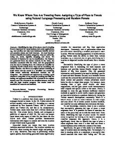
Fig. 4. The architecture of the Version 1.0 Maxelbot.
4
The Maxelbot
Our University of Wyoming “Maxelbot” (named after the two graduate students that designed and built the robot) is modular. A primary MiniDRAGON is used for control of the robot. It communicates via an I2 C bus to all other peripherals, allowing us to plug in new peripherals as needed. Figure 4 shows the architecture. The primary MiniDRAGON is the board that drives the motors. It also monitors proximity sensors and shaft encoders. The trilateration module is shown at the top of the diagram. This module controls the RF and acoustic components of trilateration. Additional modules have been built for digital compasses and thermometers. The PIC processors provide communication with the I2 C bus. The
9
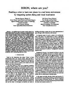
Fig. 5. The Version 1.0 Maxelbot itself.
last module is being built especially for the purpose of chemical plume tracing (i.e., following a chemical plume back to its source). It is composed of multiple chemical sensors, and sensors to measure wind speed and direction. Chemical plume tracing algorithms will run on the additional dedicated MiniDRAGON. The completed Maxelbot is shown in Figure 5.
5
Experiments and Demonstrations
The following subsections illustrate different exemplar tasks that we can perform by using the trilateration framework. It is important to note that given the small number of Maxelbots currently built (three) most of these tasks are not swarm tasks per se. Also, most of our control algorithms are currently behavior-based, and are generally not novel. However, it is important to keep in mind that the point of the demonstrations is (1) to test and debug our hardware, and (2) to show the utility and functionality of the trilateration framework. 5.1
Accuracy Experiment
To test the accuracy of the trilateration module, we placed a robot on our lab floor, with transducer B at (000 , 000 ). Then we placed an emitter along 24 grid points from (−2400 , −2400 ) to (2400 , 2400 ). The results are shown in Figure 6. The average error over all grid points is very low – 0.600 , with a minimum of 0.100 and a maximum of 1.200 . 5.2
Linear Formations
We are currently investigating the utility of linear formations of robots in corridorlike environments, such as sewers, pipes, ducts, etc. As stated above, each robot has a unique ID. Robot 0 is the leader. Robot 1 follows the leader. Robot 2 follows robot 1. Initially, the three robots are positioned in a line in the following
10 Actual vs. Perceived Location of Beacon 30 24 18 12
inches
6 0 −6 −12 −18 −24 −30 −30 −24 −18 −12 −6
0
6
12
18
24
30
inches Perceived Location
Actual Location
Receivers
Fig. 6. The perceived location of the emitter, versus the actual location.
order: robot 0, robot 1, robot 2, with robot 0 being at the head of the line. The distance between the neighboring robots is 1200 . The behavior is as follows. Robot 0 moves forward in a right curved trajectory (for the sake of making the demonstration more interesting). Robot 0 continually monitors how far behind robot 1 is. If the distance behind is greater than 14 00 , then robot 0 will stop, waiting for robot 1 to catch up. Robot 1 adjusts its own position to maintain robot 0 at coordinates (000 , 1200 ) relative to its own coordinate system. Robot 2 acts the same way with respect to robot 1 (see Figure 7). The robots maintained the correct separation very well, while moving.
Fig. 7. Three Maxelbots in linear formation.
5.3
Box/Baby Pulling
Another emphasis in our research is search and rescue. We have successfully used two robots to push (or pull) an unevenly weighted box across our lab. However,
11
the friction of the box on the floor results in slippage of the robot tires. This produces random rotations of the box. Instead, Figure 8 shows a three robot approach, where one of the robots is not in physical contact with the box.
Fig. 8. Three Maxelbots pulling a “baby” to safety.
The behavior is as follows. Three robots are initialized in a triangular formation. Robot 0 is the leading robot while the remaining two robots stay behind the leader. Robot 1 positions itself such that the leader is at (2400 , 2400 ). Robot 2 positions itself such that the leader is at (−1800 , 2400 ). The asymmetric x values are used to compensate for the 600 baseline between transducers, yielding an isosceles triangle. Robot 0 moves forward along a left curved trajectory. Robot 0 continually monitors robot 1 and robot 2. If either of the two robots falls behind, robot 0 will stop and wait for both of the robots to be within the desired distance of 3400 . Note that while robots 1 and 2 are tethered to the baby basket, robot 0 is not. Hence robot 0 (with the other two robots and the basket) follows a fairly well-controlled trajectory, subject to the limits of the accuracy of our shaft encoders and standard slippage. 5.4
Physicomimetics Formations for Chemical Plume Tracing
As a test of our hardware using a true swarm control algorithm, we implemented artificial physics (AP) on the robots [6]. Figure 9 shows three Maxelbots selforganizing into an equilateral triangle. As has been shown in prior work [6,12] a goal force can be applied to AP formations, such that the formation moves towards the goal, without breaking the formation apart. We have used a light source for our goal, and have had success using the digital compass to drive the formation in a given direction. Since one of our research thrusts is chemical plume tracing (CPT) [13], we intend to use the CPT module (described above) as our goal force. The objective of CPT is to locate the source (e.g. a leaking pipe) of a hazardous airborne plume by measuring flow properties, such as toxin concentration and wind speed. Simulation studies in [13] suggested that faster and more accurate source localization is possible with collaborating plume-tracing vehicles. We constructed the CPT module to
12
Fig. 9. Three Maxelbots using AP to self-organize into an equilateral triangle.
test this hypothesis on real ethanol plumes. In this section, we compare CPT performance of a single Maxelbot implementation against a distributed approach using three Maxelbots. As the trace chemical we employ ethanol, a volatile organic compound (VOC), and measure the chemical concentration using Figaro TGS2620 metal-oxide VOC sensors. The single Maxelbot carries four of these sensors, mounted at each corner, while there are only three chemical sensors in the distributed implementation – one sensor per Maxelbot. In both versions, the HCS12 microprocessor performs analog-to-digital conversion of sensor output, and then navigates according to a CPT strategy. We employ one of the most widely-used CPT strategies called chemotaxis, which advances the vehicle in the direction of an increasing chemical gradient. For our first experiment, we performed 23 CPT evaluation experiments in a small 60 × 110 room, using an ethanol-filled flask as the chemical source, with the single, more capable Maxelbot. The separation between the source and the starting location of the Maxelbot was 7.50 on average. Each run terminated when the Maxelbot came within 500 of the ethanol flask (a CPT success), or after 30 minutes of unsuccessful plume tracing. Of the 23 test runs, 17 were successful in locating the source (a 74% success rate), with the average localization time of 18 minutes (σt = 6.2 minutes). These results are consistent with those reported in the literature [14], although our definition of a CPT success is decidedly more stringent than the typical completion criterion used by others. For our second experiment we used a much larger 250 × 250 indoor environment. This environment is far more difficult – out of 9 trials, the single Maxelbot only succeeded twice, for a success rate of 22.2%. The variance in the time to success was very large; 3:30 and 17:30 minutes respectively (σt = 9.9 minutes). A typical movement trace is shown in Figure 10 (left). The Maxelbot’s path indicates that it is having a very difficult time following the chemical gradient in this larger environment. For our third experiment, we ran 10 experiments with the distributed Maxelbot implementation. As mentioned above, each of three Maxelbots carries only one chemical sensor. A triangular formation is maintained by the AP algorithm. Each Maxelbot shares the chemical sensor information with its neighbors, and
13
Fig. 10. Visualization of a sample CPT trace for each implementation. The large, dark rectangular blocks are obstacles (i.e., bulky laboratory equipment); the emitter is shown with the diamond shape, and each Maxelbot is depicted as a triangle. The Maxelbot path is drawn using a lightly-shaded line; for the multi-Maxelbot trace, the singular path is computed by averaging the locations of the three Maxelbots.
then each Maxelbot independently computes the direction to move. Because the formation force is stronger than the goal force, the formation remains intact, and serves as a mechanism for moving the formation along a consensus route. Despite the fact that each Maxelbot senses far less chemical information than before (and the total number of chemical sensors has decreased from four to three), performance increased markedly! Out of 10 trials, the distributed implementation successfully found the chemical source six times, for a 60% success rate. Also, this implementation showed a far more consistent source emitter approach pattern, with an average search time of just seven minutes (and σ t = 5.8 minutes). A typical path can be seen in Figure 10 (right). Snapshots of an actual run can be seen in Figure 11.
Fig. 11. Three Maxelbot CPT test run; robots are moving from left to right.
14 Metric Single Maxelbot Three Maxelbots Success Rate 22.2% 60.0% Search Time 630.0 sec (σ = 594.0) 415.0 sec (σ = 349.4) Contact Duration 532.5 sec (σ = 668.2) 677.5 sec (σ = 361.2) Table 1. CPT performance measures for both implementations: the swarm-based Maxelbot implementation outperforms the single Maxelbot version on each evaluation metric (standard deviation values are given in parenthesis).
Performance statistics for each CPT implementation are given in Table 1. Success rate is simply the percentage of trials in which a Maxelbot drove within one foot of the emitter. Search time is a measure of how long it took for the Maxelbots to find the emitter, computed for trials where the emitter was found. The contact duration is the total length of time that a Maxelbot was within one foot of the chemical emitter. To make the comparison fair for both implementations, the duration given for the Maxelbot swarm implementation includes at most one Maxelbot per time step. In practice, however, there is great value in having multiple Maxelbots near the emitter, for instance in order to identify a potential source and then extinguish it [13]. To place this in perspective, for the distributed implementation, when one Maxelbot is near the source, all three are near the source. However, if one is using the single Maxelbot implementation the success rate is 22.2%. Hence, the probability of having three of these independent non-collaborating robots near the source is approximately 1% (0.222 3 ), as opposed to a success rate of 60%.
6
Summary
This paper describes a novel 2D trilateration framework for the accurate localization of neighboring robots. The framework uses three acoustic transceivers and one RF transceiver. By also using the RF to exchange information between robots, we couple localization with data exchange. Our framework is designed to be modular, so that it can be used on different robotic platforms, and is not restricted to any particular class of control algorithms. Although we do not rely on GPS, stationary beacons, or environmental landmarks, their use is not precluded. Our framework is fully distributed, inexpensive, scalable, and robust. There are several advantages to our framework. First, the basic trilateration equations are elegant and could be implemented purely in hardware. Second, the system is well-conditioned, indicating minimal sensitivity to measurement error. Third, it should provide greater localization accuracy than IR localization methods, especially in outdoor situations. The quality of the accuracy is confirmed via empirical tests. To illustrate the general utility of our framework, we demonstrate the application of three of our robots on three different tasks: linear formations, box pulling, and geometric formation control for chemical plume tracing. The trilateration hardware performed well on all three tasks. The first two tasks utilize
15
behavior-based control algorithms, while the latter uses artificial physics (AP). The latter is especially interesting, because it demonstrates the application of a true swarm-based control algorithm. One of our primary research interests is chemical plume tracing, using AP. In order to accomplish this task, a special chemical sensing module has also been built in-house. On the third task AP is combined with the chemical sensing module to perform chemical plume tracing. Experimental results indicate that a small swarm of less capable Maxelbots easily outperforms one more capable Maxelbot. Open Source Project URL http://www.cs.uwyo.edu/∼wspears/maxelbot provides details on this project.
References 1. Borenstein, J., Everett, H., Feng, L.: Where am I? Sensors and methods for mobile robot positioning. Technical report, University of Michigan (1996) 2. Balch, T., Hybinette, M.: Social potentials for scalable multirobot formations. In: IEEE Transactions on Robotics and Automation. Volume 1. (2000) 73–80 3. Fax, J., Murray, R.: Information flow and cooperative control of vehicle formations. IEEE Transactions on Automatic Control 49 (2004) 1465–1476 4. Fierro, R., Song, P., Das, A., Kumar, V.: Cooperative control of robot formations. In Murphey, R., Pardalos, P., eds.: Cooperative Control and Optimization. Volume 66., Hingham, MA, Kluwer Academic Press (2002) 73–93 5. Brogan, D., Hodgins, J.: Group behaviors for systems with significant dynamics. Autonomous Robots 4 (1997) 137–153 6. Spears, W., Spears, D., Hamann, J., Heil, R.: Distributed, physics-based control of swarms of vehicles. Autonomous Robots 17 (2004) 137–162 7. L. Navarro-Serment, L., Paredis, C., Khosla, P.: A beacon system for the localization of distributed robotic teams. In: International Conference on Field and Service Robots, Pittsburgh, PA (1999) 232–237 8. MacArthur, D.: Design and implementation of an ultrasonic position system for multiple vehicle control. Master’s thesis, University of Florida (2003) 9. Rothermich, J., Ecemis, I., Gaudiano, P.: Distributed localization and mapping with a robotic swarm. In S ¸ ahin, E., Spears, W., eds.: Swarm Robotics, SpringerVerlag (2004) 59–71 10. Payton, D., Estkowski, R., Howard, M.: Pheromone robotics and the logic of virtual pheromones. In S ¸ ahin, E., Spears, W., eds.: Swarm Robotics, SpringerVerlag (2004) 46–58 11. Heil, R.: A trilaterative localization system for small mobile robots in swarms. Master’s thesis, University of Wyoming, Laramie, WY (2004) 12. Spears, W., Heil, R., Zarzhitsky, D.: Artificial physics for mobile robot formations. In: Proceedings IEEE International Conference on Systems, Man, and Cybernetics. (2005) 2287–2292 13. Zarzitsky, D., Spears, D., Spears, W.: Distributed robotics approach to chemical plume tracing. In: IEEE/RSJ International Conference on Intelligent Robots and Systems (IROS’05). (2005) 4034–4039 14. Lilienthal, A.: Gas Distribution Mapping and Gas Source Localisation with a Mobile Robot. PhD thesis, University of T¨ ubingen (2004)


![work is where you are - Leitz [PDF]](https://m.moam.info/img/260x300/work-is-where-you-are-leitz-pdf_64aaaf0e098a9ec4628b459a.jpg)