Oct 13, 2016 - Neural networks have drawn significant interest from the machine learning ... to show that for a given upper bound on the approx- imation error, shallow ... LG] 13 Oct 2016 ... ically, we aim to answer the following two questions. Given a ... The second question asks ...... binary step units and T3(m â. 1) (log3.
Why Deep Neural Networks?
Shiyu Liang University of Illinois Urbana-Champaign
arXiv:1610.04161v1 [cs.LG] 13 Oct 2016
Abstract Recently there has been much interest in understanding why deep neural networks are preferred to shallow networks. In this paper, we show that, for a large class of piecewise smooth functions, the number of neurons needed by a shallow network to approximate a function is exponentially larger than the corresponding number of neurons needed by a deep network for a given degree of function approximation. First, we consider univariate functions on a bounded interval and require a neural network to achieve an approximation error of ε uniformly over the interval. We show that shallow networks (i.e., networks whose depth does not depend on ε) require Ω(poly(1/ε)) neurons while deep networks (i.e., networks whose depth grows with 1/ε) require O(polylog(1/ε)) neurons. We then extend these results to certain classes of important multivariate functions. Our results are derived for neural networks which use a combination of rectifier linear units (ReLUs) and binary step units, two of the most popular type of activation functions. Our analysis builds on this simple observation that the binary approximation of a real number in the interval [0, 1] can be represented by a deep neural network which uses a “small” number of neurons.
1
Introduction
Neural networks have drawn significant interest from the machine learning community, especially due to their recent empirical successes (see the surveys (Bengio, 2009)). Neural networks are used to build stateof-art systems in various applications such as image
R. Srikant University of Illinois Urbana-Champaign
recognition, speech recognition, natural language process and others (see, Krizhevsky et al. 2012; Goodfellow et al. 2013; Wan et al. 2013, for example). The result that neural networks are universal approximators is one of the theoretical results most frequently cited to justify the use of neural networks in these applications. Numerous results have shown the universal approximation property of neural networks with one hidden layer in approximations of different function classes, (see, e.g., Cybenko 1989; Hornik et al. 1989; Hornik 1991; Chui and Li 1992; Barron 1993). All these results and many others provide upper bounds on the network size and assert that small approximation error can be achieved if the network size is sufficiently large. More recently, there has been much interest in understanding the approximation capabilities of deep versus shallow networks. Delalleau and Bengio (2011) and Telgarsky (2016) have shown that there exist deep networks which cannot be approximated by shallow networks unless they use an exponentially larger amount of units or neurons. Eldan and Shamir (2015) have shown that, to approximate a specific function, a two-layer network requires an exponential number of neurons in the input dimension, while a three-layer network requires a polynomial number of neurons. These recent papers demonstrate the power of deep networks by showing that depth can lead to an exponential reduction in the number of neurons required, for specific functions or specific neural networks. Our goal here is different: we are interested in function approximation specifically and would like to show that for a given upper bound on the approximation error, shallow networks require exponentially more neurons than deep networks for a large class of functions. The multilayer neural networks considered in this paper are allowed to use either rectifier linear units (ReLU) or binary step units (BSU), or any combination of the two. The main contributions of this paper are • We have shown that, for ε-approximation of functions with enough piecewise smoothness, a multilayer neural network which uses Θ(log(1/ε)) lay-
ers only needs O(polylog(1/ε)) neurons, while Ω(poly(1/ε)) neurons are required by neural networks with o(log(1/ε)) layers. In other words, shallow networks require exponentially more neurons than a deep network to achieve the level of accuracy for function approximation. • We have shown that for all differentiable and strongly convex functions, multilayer neural networks need Ω(log(1/ε)) neurons to achieve an εapproximation. Thus, our results for deep networks are tight. The outline of this paper is as follows. In Section 2, we present necessary definitions and the problem statement. In Section 3, we present upper bounds on network size, while the lower bound is provided in Section 4. Conclusions are presented in Section 5.
2
Preliminaries and problem statement
In this section, we present definitions on feedforward neural networks and formally present the problem statement. 2.1
• Rectifier linear unit: σ(x) = max{0, x}, x ∈ R. • Binary step unit: σ(x) = I{x ≥ 0}, x ∈ R. We call the number of layers and the number of neurons in the network as the depth and the size of the feedforward neural network, respectively. We use the set F(N, L) to denote the function set containing all feedforward neural networks of depth L, size N and constructed by rectifier linear units and binary step units. We say one feedforward neural network is deeper than the other network if and only if it has a larger depth. Through this paper, the terms feedforward neural network and multilayer neural network are used interchangeably. 2.2
In this paper, we focus on bounds on the size of the feedforward network function approximation. Specifically, we aim to answer the following two questions. Given a function f with continuous derivatives of sufficient order and an error upper bound of ε > 0, if we use a multilayer neural network f˜ of depth L and size N to approximate f , then 1 does there exist upper bounds on L(ε) and N (ε) such that
Feedforward Neural Networks
A feedforward neural network is composed of layers of computational units and defines a unique function f˜ : Rd → R. Let L denote the number of hidden layers, Nl denote the number of units of layer l, vector x = (x(1) , ..., x(d) ) denote the input of neural network, l zjl denote the output of the jth unit in layer l, wi,j denote the weight of the edge connecting unit i in layer l and unit j in layer l + 1, blj denote the bias of the unit j in layer l. Then outputs between layers of the feedforward neural network can be characterized by following iterations: ! Nl X l+1 l+1 l l zj = σ wi,j zi + bj , l ∈ [L − 1], j ∈ [Nl+1 ], i=1
with input layer:
zj1
=σ
d X
0 wi,j x(i)
+
b1j
i=1
output layer: f˜(x) = σ
NL X i=1
L L wi,j zi
+
!
,
bL+1 j
j ∈ [N1 ], !
Problem Statement
min
f˜∈F (N,L)
kf (x) − f˜(x)k ≤ ε?
2 does there exist a lower bound on N (L, ε) for a fixed depth L such that min
f˜∈F (N,L)
kf (x) − f˜(x)k ≥ ε?
The first question asks what depth and size are sufficient to guarantee an ε-approximation. The second question asks, for a fixed depth, what is the minimum size of a neural network required to guarantee an εapproximation. Obviously, tight bounds in the answers to these two questions provide tight bounds on the network size and depth required for function approximation. Besides, solutions to these two questions together can be further used to answer the following question. If a deeper neural network of size Nd and a shallower neural network of size Ns are used to approximate the same function with the same error, then how fast does the ratio Nd /Ns decay to zero as the error decays to zero?
.
Here, σ(·) denotes the activation function and [n] denotes the index set [n] = {1, ..., n}. In this paper, we only consider two important types of activation functions:
3
Upper bounds on function approximations
In this section, we present upper bounds on the size of the multilayer neural network which are sufficient
x − x0
x
≥1
≥
1 2
...
1 − 12
+
x0
+
...
2nd layer ≥
x−
: binary step unit
!n−1
xi i=1 2i
1 2n
1 − 21n xn
x1
1st layer
x1 2
≥
1 −1
x − x0 −
+
+ x−
nth layer
!n
xi i=0 2i
: adder
Figure 1: An n-layer neural network structure for finding the binary expansion of a number in [0, 1]. for function approximation. Before stating the results, some notations and terminology deserve further explanation. First, the upper bound on the network size represents the number of neurons required at most for approximating a given function with a certain error. Secondly, the notion of the approximation is the L∞ distance: for two functions f and g, the L∞ distance between these two function is the maximum point-wise disagreement over the cube [0, 1]d . 3.1
Approximation of univariate functions
In this subsection, we present all results on approximating univariate functions. We first present a theorem on the size of the network for approximating a simple quadratic function. As part of the proof, we present the structure of the multilayer feedforward neural network used and show how the neural network parameters are chosen. Results on approximating general functions can be found in Theorem 2 and Theorem 1. For function f (x) = x2 , x ∈ [0, 1], there exists a multilayer �neural network f˜(x) with � 1 O log ε �layers, O log 1ε binary step units and O log 1ε rectifier linear units such that |f (x) − f˜(x)| ≤ ε,
x ∈ [0, 1].
Proof. The proof is composed of three parts. For any x ∈ [0, 1], we first use the multilayer neural network Pn to approximate x by its finite binary expansion i=0 x2ii . We then construct the � neural network to imPna 2-layer xi plement function f i=0 2i . For each x ∈ P [0, 1], x can be denoted by its binary ex∞ pansion x = i=0 x2ii , where xi ∈ {0, 1} for all i ≥ 0. It is straightforward to see that the n-layer neural network shown in Figure 1 can be used to find x0 , ..., xn .
Pn xi � Next, we implement the function f˜(x) = f i=0 2i by a two-layer neural network. Since f (x) = x2 , we then rewrite f˜(x) as follows: !2 n n n X X X xi xj xi · 1 f˜(x) = = i i 2 2 2j i=0 i=0 j=0 n n X X 1 xj = max 0, 2(xi − 1) + i 2 2j j=0 i=0
The third equality follows from the fact that xi ∈ {0, 1} for all i. Therefore, the function f˜(x) can be implemented by a multilayer network containing a deep structure shown in Figure 1 and another hidden layer with n rectifier linear units. This multilayer neural network has n + 2 layers, n binary step units and n rectifier linear units. Finally, we consider the approximation error of this multilayer neural network, !2 n n X X 2 x x i i ≤ 2 x − |f (x) − f˜(x)| = x − i i 2 2 i=0 i=0 n ∞ ∞ X x X x X xi 1 i i = 2 − ≤ n−1 = 2 i i i 2 2 2 2 i=0 i=0 i=n+1
Therefore, in order to achieve er� ε-approximation � ror, one should choose n = log2 1ε + 1. �In sum1 mary, the � deep neural network has O log ��ε layers, 1 1 O log ε binary step units and O log ε rectifier linear units. Next, a theorem on the size of the network for approximating general polynomials is given as follows. Pp i Theorem 2. P For polynomials f (x) = i=0 ai x , p x ∈ [0, 1] and i=1 |ai | ≤ 1, there exists a multi-
� layer neural network f˜(x) with O p + log �pε layers, � O log pε binary step units and O p log pε rectifier linear units such that |f (x) − f˜(x)| ≤ ε,
x ∈ [0, 1].
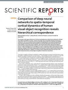
Proof. The proof is composed of three parts. We first use the deep structure shown in Figure 1 to find the Pn n-bit binary expansion i=0 ai xi of x. Then we construct a multilayer network to approximate polynomials gi (x) = xi , i = 1, ..., p. Finally, we analyze the approximation error. Using the same deep structure shown in Figure 1, we could find the binary expansion sequence {x0 , ..., xn }. In this step, we used Pnn binary steps units in total. Now we rewrite gm+1 ( i=0 2xni ), ! ! n n n X X X xj xi xi gm+1 = gm · i i 2 2 2j j=0 i=0 i=0 !# " n n X X xi 1 = xj · j gm 2 2i i=0 j=0 ! # " n n X X xi = , 0 (1) max 2(xj − 1) + gm 2i j=0 i=0 Clearly, the equation (1) defines iterations between the outputs of neighbor layers. Therefore, the deep neural network shown in Figure 2 can be used to implement the iteration given by (1). Further, to implement this network, one should use p layers with pn rectifier linear units in total. We now define the output of the multilayer neural network as p n X X x j f˜(x) = ai gi . j 2 i=0 j=0
For this multilayer network, the approximation error is X p n X X p xj i |f (x) − f˜(x)| = − a x ai gi i j 2 i=0 j=0 i=0 p n X X xj i |ai | · gi ≤ − x j 2 i=0 j=0 X p X n xj ≤ p i|ai | · − x = j 2 2n−1 j=0 i=0
This indicates, to achieve � � ε-approximation error, one should choose n = log pε + 1. Besides, since we used n+p layers with n binary step units and pn rectifier linear units in total, network thus � this multilayer neural � has O p + log�pε layers, O log pε binary step units and O p log pε rectifier linear units.
In Theorem 2, we have shown an upper bound on the size of multilayer neural network for approximating polynomials. We can easily observe that the number of neurons in network grows as p log p with respect to p, the degree of the polynomial. We note that both Andoni et al.(2014) and Barron(1993) showed the sizes of the networks in grow exponentially with respect to p if only 3-layer neural networks are allowed to use in approximating polynomials. Besides, every function f with p + 1 continuous derivatives on a bounded set can be approximated easily with a polynomial with degree p. This is shown by the following well known result of Lagrangian interpolation. By this result, we could further generalize Theorem 2. The proof can be found in the reference (Gil et al., 2007). Lemma 3 (Lagrangian interpolation at Chebyshev points). If a function f is defined at points z0 , ..., zn , zi = cos((k + 1/2)π/(n + 1)), i ∈ [n], there exists a polynomial of degree not more that n such that Pn (zi ) = f (z i = 0, ..., n. This polynomial is given Pi ), n by Pn (x) = i=0 f (zi )Li (x) where Li (x) =
n Y πn+1 (x) and π (x) = (x − zj ). n+1 (x − zi )π 0 (zi ) j=0
Additionally, if f is continuous on [−1, 1] and n + 1 times differentiable in (−1, 1), then kRn k = kf − Pn k ≤
1
(n+1)
f
, 2n (n + 1)!
where f (n) (x) is the derivative of f of the nth order and the norm kf k is the l∞ norm kf k = maxi∈[−1,1] f (x). Then the upper bound on the network size for approximating more general functions follows directly from Theorem 2 and Lemma 3. Theorem 4.� Assume � that function f is continuous on [0, 1] and log 2ε + 1 times differentiable in (0, 1). Let f (n) denote the the derivative
(n)of f of nth order
f ≤ n! holds for and kf k��= max f (x). If x∈[0,1] � � 2 all n ∈ log ε + 1 , then there exists a deep neural � � network f�˜ with O �log 1ε layers, O log 1ε binary step �2 units, O log 1ε rectifier linear units such that |f (x) − f˜| ≤ ε
for ∀x ∈ [0, 1].
� � Proof. Let N = log 2ε . From Lemma 3, it follows that there exists polynomial PN of degree N such that for any x ∈ [0, 1],
(N +1)
f
1 |f (x) − PN (x)| ≤ N ≤ N. 2 (N + 1)! 2
x0
xn
xn
x2
x0 x1 x2
x0 x1
ReLU
xn
x2
ReLU
ReLU
...
... ReLU
+
ReLU
xn
gp
!
...
xn
n " xi i=0
2i
#
ReLU
ReLU
ReLU
+!
g1
n " xi i=0
2i
#ReLU
...
...
...
1
x2
xn
ReLU
xn
ReLU
xn
x2
...
ReLU
x1
...
...
...
...
xn
x1
ReLU
ReLU
x2
x0
...
x2
x1
x0
...
...
x1
x1
x0 x1 x2
x0
...
x0
x0 x1 x2
+!
g2
n " xi i=0
2i
#ReLU
+!
g3
n " xi i=0
2i
#
+!
gp−2
n " xi i=0
2i
#ReLU
+ gp−1
!
n " xi i=0
2i
#
Figure 2: The implementation of polynomial function Let x0 , ..., xN denote the first N + 1 bits of the binary expansion of x and define ! N X xi ˜ f (x) = PN . 2N i=0 In the following, we first analyze the approximation error of f˜ and next P show the implementation of this N xi function. Let x ˜ = i=0 2i . The error can now be upper bounded by |f (x) − f˜(x)| = |f (x) − PN (˜ x)|
≤ |f (x) − f (˜ x)| + |f (˜ x) − PN (˜ x)| N
X xi 1 1 1
+ N ≤ N + N ≤ε ≤ f (1) · x − i 2 2 2 2 i=0
In the following, we describe the implementation of f˜ by a multilayer neural network. Since PN is a polynomial of degree N , function f˜ can be rewritten as ! ! N N N X X X x x i i f˜(x) = PN = cn gn 2i 2i n=0 i=0 i=0 for some coefficients c0 , ..., cN and gn = xn , n ∈ [N ]. Hence, the multilayer neural network shown in the Figure 2 can be used to implement f˜(x). Notice that the network uses N layers with N binary step units in total to decode x0 ,...,xN and N layers with N 2 rectifier linear units in total� to construct the polynomial PN . � Substituting N = log 2ε , we have proved the theorem. Theorem 4 shows that any function f with enough smoothness can be approximated �by a multilayer neural network containing polylog 1ε neurons with ε error. Further, Theorem 4 can be used to show that for functions h1 ,...,hk with enough smoothness, then linear combinations, multiplications and compositions of
these functions can as well be approximated� by multilayer neural networks containing polylog 1ε neurons with ε error. Specific results are given in the following corollaries. Corollary 5 (Function addition). Suppose that all functions h1 , ..., hk satisfy the conditions in Theorem 4, and the vector β ∈ {ω ∈ Rk : kωk1 = 1}, Pk then for the linear combination f = i=1 βi hi , there � exists a deep neural network f˜� with O �log 1ε layers, � �2 O log 1ε binary step units, O log 1ε rectifier linear units such that |f (x) − f˜| ≤ ε
for ∀x ∈ [0, 1].
Remark: Clearly, Corollary 5 follows directly from the fact that the linear combination f satisfies the conditions in Theorem 4 if all the functions h1 ,...,hk satisfy those conditions. We note here that the upper bound on the network size for approximating linear combinations is independent of k, the number of component functions. Corollary 6 (Function multiplication). Suppose that all � functions h1 ,...,hk are � continuous on [0, 1] and 4k log2 4k + 4k + 2 log2 2ε + 1 times differentiable (n) in (0, 1). ��If khi k ≤ n! holds �for �all i ∈ [k] and n ∈ 4k log2 4k + 4k + 2 log2 2ε + 1 then for Qk the multiplication f = i=1 hi , there exists a � multilayer neural network� f˜ with O k log k + log 1ε layers, O k log k + log�1ε binary step units and � �2 O (k log k)2 + log 1ε such that |f (x) − f˜(x)| ≤ ε,
for ∀x ∈ [0, 1].
Corollary 7 (Function composition). Suppose that all functions h1 , ..., hk : [0, 1] → [0, 1] satisfy the conditions in Theorem 4, then for the composition f = h1 ◦h2 ◦...◦h�k , there exists a multilayer neural net� � 1 1 2 ˜ work f with O k log k log ε + log k log ε layers,
� �2 � O k log k log 1ε + log k log 1ε binary step units and � � � � 2 4 rectifier linear units such O k 2 log 1ε + log 1ε that |f (x) − f˜(x)| ≤ ε, for ∀x ∈ [0, 1]. Remark: Proofs of Corollary 6 and 7 can be found in the appendix. We observe that different from the case of linear combinations, the upper bound on the network size grows as k 2 log2 k in the case of function �2 multiplications and grows as k 2 log 1ε in the case of function compositions where k is the number of component functions. � In this sbsection, we have shown a polylog 1ε upper bound on the network size for ε-approximation of both univariate polynomials and general univariate functions with enough smoothness. Besides, we have shown that linear combinations, multiplications and compositions of univariate functions with enough smoothness can as well be approximated with ε �error by a multilayer neural network of size polylog 1ε . In the next subsection, we will show the upper bound on the network size for approximating multivariate functions. 3.2
Approximation of multivariate functions
In this subsection, we present all results on approximating multivariate functions. We first present a theorem on the upper bound on the neural network size for approximating a product of multivariate linear functions. We next present a theorem on the upper bound on the neural network size for approximating general multivariate polynomial functions. Finally, similar to the results in the univariate case, we present the upper bound on the neural network size for approximating the linear combination, the multiplication and the composition of multivariate functions with enough smoothness. d Theorem Qp8. LetT W� = {w ∈ Rd f (x) = i=1 wi x , x ∈ [0, 1] 1, ..., � p, there �exists a deep neural �
: kwk1 = 1}. For and wi ∈ W , i = network f˜(x) with �
O p + log pd layers and O log pd binary step units ε ε � � and O pd log pd rectifier linear units such that ε |f (x) − f˜(x)| ≤ ε,
∀x ∈ [0, 1]d .
Theorem 8 shows an upper bound on the network size for ε-approximation of a product of multivariate linear functions. Furthermore, since any general multivariate polynomial can be viewed as a linear combination of products, the result on general multivariate polynomials directly follows from Theorem 8.
Theorem 9. Let the multi-index vector α = (α1 , ..., αd ), the norm |α| = α1 +...+αd , the coefficient Cα = Cα1 ...αd , the input vector x = (x(1) , ..., x(d) ) α1 (d) αd . For posiand the multinomial xα = x(1) ...xP tive integer p and polynomial f (x) = α:|α|≤p Cα xα , P x ∈ [0, 1]d and α:|α|≤p |Cα | ≤ 1, there exists a deep � � neural network f˜(x) of depth O p + log dp and size ε
˜ ≤ ε, where N (d, p, ε) such that |f (x) − f (x)|
N (d, p, ε) = p2
�
� pd p+d−1 log . d−1 ε
Remark: The proof is given in the appendix. By further analyzing the results on the network size, we obtain the following �results: (a) fixing degree p, N (d, ε) = O dp+1 log dε as d → ∞ and � (b) fixing p d input dimension d, N (p, ε) = O p log ε as p → ∞. Similar results on approximating multivariate polynomials were obtained by Andoni et al.(2014) and Barron(1993). Barron(1993) showed that on can use a 3-layer neural network to approximate any multivariate polynomial with degree p, dimension d and network size dp /ε2 . Andoni et al.(2014) showed that one could use the gradient descent to train a 3-layer neural network of size d2p /ε2 to approximate any multivariate polynomial. However, Theorem 9 shows that the deep neural network could reduce the network size � from O (1/ε) to O log 1ε for the same ε error. Besides, for a fixed input dimension d, the size of the 3layer neural network used by Andoni et al.(2014) and Barron(1993) grows exponentially with respect to the degree p. However, the size of the deep neural network shown in Theorem 9 grows only polynomially with respect to the degree. Therefore, the deep neural network could reduce the network size from O(exp(p)) to O(poly(p)) when the degree p becomes large. Theorem 9 shows an upper bound on the network size for approximating multivariate polynomials. Further, by combining Theorem 4 and Corollary 7, we could obtain an upper bound on the network size for approximating more general functions. The results are shown in the following corollary. Corollary 10. Assume that all univariate functions h1 , ..., hk : [0, 1] → [0, 1], k ≥ 1, satisfy the conditions in Theorem 4. Assume that the multivariate polynomial l(x) : [0, 1]d → [0, 1] is of degree p. For composition f = h1 ◦ h2 ◦ ... ◦ hk ◦ l(x), there exists a multilayer neural network �f˜ of � �2 depth O p + log d + k log k log 1ε + log k log 1ε and ˜ of size N (k, p, d, ε) such that |f (x) − f (x)| ≤ ε for
∀x ∈ [0, 1]d , where
� � � pd 2 p+d−1 N (k, p, d, ε) = O p log d−1 ε � �2 � �4 ! 1 1 +k 2 log + log ε ε
Remark: Corollary 10 shows an upper bound on network size for approximating compositions of multivariate polynomials and general univariate functions. The upper bound can be loose due to the assumption that l(x) is a general multivariate polynomials of degree p. For some specific cases, the upper bound can be much smaller. We present two specific examples in Corollary 11 and Corollary 12. Corollary 11 (Gaussian function). For Gaussian Pd (i) 2 function f (x) = f (x(1) , ..., x(d) ) = e− i=1 (x ) /2 , x ∈ [0, 1]d , there exists a deep� neural network f˜(x) � d d layers, with O log ε � �O d log ε binary step units and � 2 O d log dε + log 1ε rectifier linear units such that |f˜(x) − f (x)| ≤ ε for ∀x ∈ [0, 1]d .
Corollary 12 (Ridge function). If f (x) = g(aT x) for some direction a ∈ Rd with kak1 = 1, a � 0, x ∈ [0, 1]d and some univariate function g satisfying conditions in Theorem 4, then there � exists a multilayer � neural network f˜ with �O log 1ε � layers, O log 1ε bi�2 nary step units and O log 1ε rectifier linear units such that |f (x) − f˜(x)| ≤ ε for ∀x ∈ [0, 1]d .
In this subsection, we have shown that a similar � polylog 1ε upper bound on the network size for εapproximation of general multivariate polynomials and functions which are compositions of univariate functions and multivariate polynomials. The results in this section can be used to� find a multilayer neural network of size polylog 1ε which provides an approximation error of at most ε. In the next section, we will present lower bounds on the network size for approximating both univariate and multivariate functions. The lower bound together with the upper bound shows a tight bound on the network size required for function approximations. While we have presented results in both the univariate and multivariate cases for smooth functions, the results automatically extend to functions that are piecewise smooth, with a finite number of pieces. In other words, if the domain of the function is partitioned into regions, and the function is sufficiently smooth (in the sense described in the Theorems and Corollaries earlier) in each of the regions, then the results essentially remain unchanged except for an additional factor which will depend on the number of regions in the domain.
4
Lower bounds on function approximations
In this section, we present lower bounds on the network size in function for certain classes of functions. Next, by combining the lower bounds and the upper bounds shown in the previous section, we could analytically show the advantages of deeper neural networks over shallower ones. The theorem below is inspired by a similar result in for univariate quadratic functions, where it is stated without a proof. Here we show that the result extends to general multivariate strongly convex functions. Theorem 13. Assume function f : [0, 1]d → R is differentiable and strongly convex with parameter µ. Assume the multilayer neural network f˜ is composed of rectifier linear units and binary step units. If |f (x) − f˜(x)| ≤ ε
for ∀x ∈ [0, 1],
then the depth L and the network size N should satisfy 1 � µ � 2L . N ≥L 16ε This indicates the following network size should satisfy � µ � N ≥ log2 . 16ε Proof. We first prove the univariate case d = 1. The proof is composed of two parts. We say the function g(x) has a break point at x = z if g is discontinuous at z or its derivative g 0 is discontinuous at z. Then we present the proof. We first present the lower bound on the number of break points M (ε) that the multilayer neural network f˜ should have for ε-approximation of function f with error ε. We next relate the number of break points M (ε) to the network depth L and the size N . Now we calculate the lower boundpon M (ε). We first define 4 points x0 , x1 =px0 + 2 ρε/µ, x2 = x1 + p 2 ρε/µ and x3 = x2 + 2 ρε/µ, ∀ρ > 1. We assume 0 ≤ x0 < x1 < x2 < x3 ≤ 1.
We now prove that if multilayer neural network f˜ has no break point in [x1 , x2 ], then f˜ should have a break point in [x0 , x1 ] and a break point in [x2 , x3 ]. We prove this by contradiction. We assume the neural network f˜ has no break points in the interval [x0 , x3 ]. Since f˜ is constructed by rectifier linear units and binary step units and has no break points in the interval [x0 , x3 ], then we f˜ should be a linear function in the interval [x0 , x3 ], i.e., f˜(x) = ax + b, x ∈ [x0 , x3 ] for some a and b. By assumption, since f˜ approximates f with error at most ε everywhere in [0, 1], then |f (x1 ) − ax1 − b| ≤ ε
and
|f (x2 ) − ax2 − b| ≤ ε.
Now we consider the multivariate case d > 1. Assume input vector to be x = (x1 , ..., x(d) ). We now fix x(2) , ..., x(d) and define two univariate functions
Then we have f (x2 ) − f (x1 ) − 2ε f (x2 ) − f (x1 ) + 2ε ≤a≤ . x2 − x1 x2 − x1
g(y) = f (y, x(2) , ..., x(d) ), and g˜(y) = f˜(y, x(2) , ..., x(d) ).
By strong convexity of f , f (x2 ) − f (x1 ) µ + (x2 − x1 ) ≤ f 0 (x2 ). x2 − x1 2
By assumption, g(y) is a strongly convex function with parameter µ and for all y ∈ [0, 1], |g(y) − g˜(y)| ≤ ε. Therefore, by results in the univariate case, we should have
Besides, since ρ > 1 and 2ρε 2ε µ √ (x2 − x1 ) = ρµε = > , 2 x2 − x1 x2 − x1 then
a ≤ f 0 (x2 ).
N ≥L (2)
1 � µ � 2L 16ε
and N ≥ log2
� µ � . 16ε
Now we have proved the theorem.
0
Similarly, we can obtain a ≥ f (x1 ). By our assumption that f˜ = ax + b, x ∈ [x0 , x3 ], then
Remark: Theorem 13 shows that all strongly convex cannot be approximated with error ε by any multilayer neural network with rectifier linear units and bi= f (x3 ) − f (x2 ) − a(x3 − x2 ) + f (x2 ) − ax2 − b nary step units and of size smaller than log2 (µ/ε) − 4. µ ≥ f 0 (x2 )(x3 − x2 ) + (x3 − x2 )2 − a(x3 − x2 ) − ε Theorem 13 together with Theorem 1 directly shows 2 �2 that to approximate quadratic function f (x) = x2 with � µ� p 0 = (f (x2 ) − a)(x3 − x2 ) + 2 ρε/µ − ε error ε, the network size should be of order Θ log 1ε . 2 Further, by combining Theorem 13 and Theorem 4, we ≥ (2ρ − 1)ε > ε could analytically show the benefits of deeper neural networks. The result is given in the following corollary. The first inequality follows from strong convexity of f and f (x2 ) − ax2 − b ≥ ε. The second inequality Corollary 14. Assume that univariate function f satfollows from the inequality (2), while the third follows isfies conditions in both Theorem 4 and Theorem � 13. If from ρ > 1. Therefore, this leads to the contradiction. a neural network f˜s is of depth Ls = o log 1ε , size Ns Thus there exists a break point in the interval [x2 , x3 ]. and |f (x)− f˜s (x)| ≤ ε, for ∀x ∈ [0, 1], then there�exists Similarly, we could prove there exists a break point in a deeper neural network f˜d (x) of depth Θ log 1ε , size the interval [x0 , x1 ]. These indicates that to achieve εNd = O(L2s log2 Ns ) such that approximation in [0, 1],lthe multilayer neural network m q µ f˜ should have at least 41 ρε break points in [0, 1]. |f (x) − f˜d (x)| ≤ ε for ∀x ∈ [0, 1]. Therefore, � r � Remark: Corollary 14 shows that in the approxima1 µ M (ε) ≥ , ∀ρ > 1. tion of the same function, the size of the deep neu4 ρε ral network Ns is only of polynomially logarithmic orFurther, Telgarsky (2016) has shown that the maxider of the size of the shallow neural network Nd , i.e., mum number of break points that a multilayer neural Nd = O(polylog(Ns )). Similar results can be obtained network of depth L and size N could have is (N/L)L . for multivariate functions on the type considered in Thus, L and N should satisfy Section 3.2. � r � 1 µ , ∀ρ > 1. (N/L)L > 4 ρε 5 Conclusions f (x3 ) − f˜(x3 ) = f (x3 ) − ax3 − b
Therefore, we have 1 � µ � 2L N ≥L . 16ε
Besides, let m = N/L. Since each layer in network should have at least 2 neurons, i.e., m ≥ 2, then � µ � � µ � m N= log2 ≥ log2 . 2 log2 m 16ε 16ε
In this paper, we have shown that an exponentially large number of neurons are needed for function approximation using shallow networks, when compared to deep networks. The results are established for a large class of smooth univariate and multivariate functions. Our results are established for the case of feedforward neural networks with ReLUs and binary step units.
Appendix A
Proof of Corollary 5
Proof. By Theorem 4, for each hi , i = 1, ..., k, there ˜ i such that |hi (x)− exists a multilayer neural network h ˜ h(x)| ≤ ε for any x ∈ [0, 1]. Let k X
f˜(x) =
˜ i (x). βi h
i=1
Then the approximation error is upper bounded by k k X X ˜ |f (x)−f˜(x)| = βi hi (x) ≤ |βi |·|hi (x)−h(x)| = ε. i=1
where gj (x) = xj , then f˜ should has a form of ! k N N X X X x i f˜(x) = βi cij gj i 2 i=1 j=0 i=0 and can be further rewritten as " k ! N X X f˜(x) = cij βi · gj j=0
,
i=1
c0j gj
j=0
P
N X xi i=0
2i
!
N X xi i=0
2i
!#
,
where c0j = i cij βi . Therefore, f˜ can be implemented by a multilayer neural network shown � in Figure 2 and � 1 1 this network has at most O log ε layers, O log ε � � �2 binary step units, O log 1ε rectifier linear units.
Appendix B
Proof of Corollary 6
Proof. Since f (x) = h1 (x)h2 (x)...hk (x), then the derivative of f of order n is X n! (α ) (α ) (α ) f (n) = h1 1 h2 2 ...hk k . α !α !...α ! 1 2 k α +...+α =n 1 k α1 ≥0,...,αk ≥0
(α ) By the assumption that hi i ≤ αi ! holds for i = 1, ..., k, then we have
X n!
(n)
(α1 ) (α2 ) (αk )
f ≤
h1 h2 ...hk α1 !α2 !...αk ! α +...+α =n 1 k α1 ≥0,...,αk ≥0
≤
�
Since the right hand has an asymptotic order of � � � �k−1 1 e(N + k) 1 N +k p → 2N k − 1 k−1 2N 2π(k − 1)
as N → ∞, then the error has an asymptotic upper bound of
i=1
Now we compute the multilayer neural net� size� of theP N work f˜. Let N = log 2ε and i=0 x2ii be the binary ˜ i (x) has a form of expansion of x. Since h ! N N X X x i ˜ i (x) = , cij gj h 2i j=0 i=0
N X
Then from Theorem 4, it follows that there exists a polynomial of PN degree N that
(N +1) � �
f
1 N +k kRN k = kf − PN k ≤ ≤ N . k−1 (N + 1)!2N 2
� n+k−1 n!. k−1
kRN k ≤
ε (eN )k ≤ 22k+k log2 N −N ≤ . 2N 2
(3)
Since we need to choose N such that 2 N ≥ k log2 N + 2k + log2 , ε and then N can be chosen such that N ≥ 2k log2 N
2 and N ≥ 4k + 2 log2 . ε
Further function l(x) = x/ log2 x is monotonically increasing on [e, ∞) and 4k log2 4k log2 4k + log2 log2 4k 4k log2 4k ≥ log2 4k + log2 4k = 2k.
l(4k log2 4k) =
Therefore, to suffice the inequality (3), one should should choose 2 N ≥ 4k log2 4k + 4k + 2 log2 . ε � � 2 Since N = 4k log2 4k + 4k + 2 log2 ε by assumptions, then there exists a polynomial PN of degree N such that ε kf − PN k ≤ . 2 PN Let i=0 x2ii denote the binary expansion of x and let ! N X xi ˜ f (x) = PN . 2i i=0 The approximation error is ! N X x i |f˜(x) − f (x)| ≤ f (x) − f i 2 i=0 ! ! N N X xi X xi + f − PN 2i 2i i=0 i=0 N X xi ε ≤ kf (1)k x − + ≤ε 2i 2 i=0
Further, function f˜ can be implemented by a multilayer neural network shown in Figure 2 and this network has at most O(N ) layers, O(N ) binary step units and O(N 2 ) rectifier linear units.
Appendix C
Proof of Corollary 7
Proof. We prove this theorem by induction. Define function Fm = h1 ◦ ... ◦ hm , m = 1, ..., k. Let m m �2 m T1 (m) log3 3ε , T2 (m) log3 3ε and T3 (m) log3 3ε denote the number of layers, the number of binary step units and the number of rectifier linear units required at most for ε-approximation of Fm , respectively. By Theorem 4, for m = 1, there exists a multilayer neural network F˜1 with at most T1 (1) log3 3ε layers, �2 T2 (1) log3 3ε binary step units and T3 (1) log3 3ε rectifier linear units such that |F1 (x) − F˜1 (x)| ≤ ε,
for x ∈ [0, 1].
Now we consider the cases for 2 ≤ m ≤ k. We assume for Fm−1 , there exists a multilayer neural netm work F˜m−1 with not more than T1 (m − 1) log3 3ε laym ers, T2 (m − 1) log3 3ε binary step units and T3 (m − � m 2 rectifier linear units such that 1) log3 3ε ε |Fm−1 (x) − F˜m−1 (x)| ≤ , 3
for x ∈ [0, 1].
Further we assume the derivative of Fm−1 has an upper
0
≤ 1. Then for Fm , since Fm (x) can be bound Fm−1 rewritten as Fm (x) = Fm−1 (hm (x)),
˜ m with and there exists a multilayer neural network h 3 3 at most T1 (1) log3 ε layers, T2 (1) log3 ε binary step �2 units and T3 (1) log3 3ε rectifier linear units such that ˜ m (x)| ≤ ε , |hm (x) − h 3
for x ∈ [0, 1],
˜ and h m ≤ (1 + ε/3). Then for cascaded multilayer � � 1 ˜ neural network F˜m = F˜m−1 ◦ 1+ε/3 hm , we have
!
˜m h
k Fm − F˜m k = Fm−1 (hm ) − F˜m−1
1 + ε/3
!
˜m h
≤ Fm−1 (hm ) − Fm−1
1 + ε/3
! !
˜m ˜m h h
+ Fm−1 − F˜m−1
1 + ε/3 1 + ε/3
˜m
0 h
ε
≤ Fm−1 · hm −
+
1 + ε/3 3
0 ˜ m
· ≤ Fm−1
hm − h
0 ε/3
˜ m + ε
· + Fm−1 h
1 + ε/3 3 ε ε ε ≤ + + =ε 3 3 3 In addition, the derivative of Fm can be upper bounded by
0 0
· kh0m k = 1. kFm k ≤ Fm−1
Since the multilayer neural network F˜m is constructed ˜ m, by cascading multilayer neural networks F˜m−1 and h then the iterations for T1 , T2 and T3 are 3m 3m 3 =T1 (m − 1) log3 + T1 (1) log3 , ε ε ε (4) 3m 3m 3 T2 (m) log3 =T2 (m − 1) log3 + T2 (1) log3 , ε ε ε (5) � �2 � �2 3m 3m T3 (m) log3 =T3 (m − 1) log3 ε ε � �2 3 + T3 (1) log3 . (6) ε T1 (m) log3
From iterations (4) and (5), we could have for 2 ≤ m ≤ k, 1 + log3 (1/ε) m + log3 (1/ε) 1 + log3 (1/ε) ≤ T1 (m − 1) + T1 (1) m 1 + log3 (1/ε) T2 (m) = T2 (m − 1) + T2 (1) m + log3 (1/ε) 1 + log3 (1/ε) ≤ T2 (m − 1) + T2 (1) m T1 (m) = T1 (m − 1) + T1 (1)
and thus �
1 T1 (k) = O log k log ε
�
,
�
1 T2 (k) = O log k log ε
�
.
˜ l = 1, ..., p − 1 into then we can rewrite gl+1 (x),
From the iteration (6), we have for 2 ≤ m ≤ k, �
1 + log3 (1/ε) T3 (m) = T3 (m − 1) + T3 (1) m + log3 (1/ε) (1 + log3 (1/ε))3 , ≤ T3 (m − 1) + m2
�2
and thus �
T3 (k) = O
1 log ε
�2 !
Proof of Theorem 8
Proof. The proof is composed of two parts. As before, we first use the deep structure shown in Figure 1 to find the binary expansion of x and next use a multilayer neural network to approximate the polynomial. Let x = (x(1) , ..., x(d) ) and wi = (wi1 , ..., wid ). We could now use the deep structure shown in Figure 1 to find the binary expansion for each x(k) , k ∈ [d]. Let Pn x(k) x ˜(k) = r=0 2rr denote the binary expansion of x(k) , (k) where xr is the rth bit in the binary expansion of x(k) . Obviously, to decode all the n-bit binary expansions of all x(k) , k ∈ [d], we need a multilayer neural network with n layers and dn binary units in total. ˜ = (˜ Besides, we let x x(1) , ..., x ˜(d) ). Now we define
˜ = f˜(x) = f (x)
p d Y X
i=1
wik x ˜
(k)
k=1
!
.
We further define
˜ = gl (x)
l d Y X
i=1
wik x ˜
(k)
k=1
!
.
Since for l = 1, ..., p − 1, ˜ = gl (x)
l d Y X
i=1
k=1
wik x ˜
(k)
!
≤
l Y
i=1
i=1
k=1
(k)
wik x ˜
!
=
d h i X ˜ w(l+1)k x ˜(k) · gl (x)
k=1
�) n � X ˜ (k) gl (x) = w(l+1)k xr · r 2 r=0 k=1 ( �) � d n X X ˜ g ( x) l ,0 = w(l+1)k max 2(x(k) r − 1) + 2r r=0 d X
(
k=1
.
Therefore, to � approximate f = Fk , �we need �2 at most O k log k log 1ε + log k log 1ε layers, � � � 1 2 1 O k log k log ε + log k log ε binary step units � � � � 2 4 rectifier linear units. and O k 2 log 1ε + log 1ε
Appendix D
˜ = gl+1 (x)
l+1 X d Y
kwi k1 = 1,
(7)
Obviously, equation (7) defines a relationship between the outputs of neighbor layers and thus can be used to implement the multilayer neural network. In this implementation, we need dn rectifier linear units in each layer and thus dnp rectifier linear units. Therefore, to implement function f˜(x), we need p + n layers, dn binary step units and dnp rectifier linear units in total. In the rest of proof, we consider the approximation error. Since for k = 1, ..., d and ∀x ∈ [0, 1]d , p p p Y ∂f (x) X X � T ≤ = wjk · w x |wjk | ≤ p, i ∂x(k) j=1 j=1 i=1,i6=j then
˜ ≤ k∇f k2 · kx − xk ˜ 2 |f (x) − f˜(x)| = |f (x) − f (x)| pd ≤ n. 2 l m By choosing n = log2 pd ε , we have ˜ ≤ ε. |f (x) − f (x)|
Since we use nd binary step units to convert the input to binary form and dnp �neurons �in function approximation, we thus use O d log pd binary step units ε � � rectifier linear units in total. In adand O pd log pd ε dition, since we have used n layers to convert the input to binary form and p layers in the function approximation section of the� network, the whole deep structure � has O p + log pd layers. ε
Appendix E
Proof of Theorem 9
Proof. For each multinomial function g with multiindex α, gα (x) = xα , it follows from Theorem 4 that � there exists � a deep neural� network g˜α �of size and depth O |α| + log |α|d such O |α| log |α|d ε ε that |gα (x) − g˜α (x)| ≤ ε.
Let the deep neural network be X f˜(x) = Cα g˜α (x), α:|α|≤p
and thus |f (x) − f˜(x)| ≤
X
α:|α|≤p
|Cα | · |gα (x) − g˜α (x)| = ε.
Since the total number of multinomial is upper bounded by � � p+d−1 p , d−1
the size of deep neural network is thus upper bounded by � � pd p+d−1 (8) p2 log . d−1 ε
If the dimension of the input d is fixed, then (8) is has the order of � � � � pd pd d+1 2 p+d−1 = O (ep) log , p→∞ p log d−1 ε ε
while if the degree p is fixed, then (8) is has the order of � � � � pd pd p+d−1 p p2 log = O p2 (ed) log , d → ∞. d−1 ε ε
By inequalities (9) and (10), the the approximation error is upper bounded by |f (x) − f˜(x)| ! Pd Pd (i) ˜i (x(i) ) −( i=1 x )/2 ˆ i=1 g = e −f 2 Pd (i) Pd (i) ≤ e−( i=1 x )/2 − e−( i=1 g˜i (x ))/2 ! Pd Pd ˜i (x(i) ) −( i=1 g˜i (x(i) ))/2 ˆ i=1 g + e −f 2 ε ε ≤ + = ε. 2 2
� Now the deep neural network has O log dε � layers, O d log dε � binary step units and � �2 O d log dε + log 1ε rectifier linear units.
Appendix G
Proof of Corollary 12
Proof. Let t = aT x. Since kak1 = 1, a � 0 and x ∈ [0, 1]d , then 0 ≤ t ≤ 1. Then from Theorem 4, it follows that then there neural � exists a multilayer � 1 1 layers, O log binary step network g˜ with O log ε ε � � � 1 2 rectifier linear units such that units and O log ε |g(t) − g˜(t)| ≤ ε,
Appendix F
Proof of Corollary 11
Proof. It follows from the Theorem 4 that there exists d multilayer neural networks g˜1�(x(1) ), ..., g˜d (x(d) ) with � d O log ε layers and O d log dε binary step units and � O d log dε rectifier linear units in total such that x(1) 2 + ... + x(d) 2 g˜1 (x(1) ) + ... + g˜d (x(d) ) ε − ≤ . 2 2 2 (9) Besides, from Theorem 4, it follows that there exists a� � 1 1 deep neural network fˆ with O log layers O log ε � �2 � ε binary step units and O log 1ε such that ε |e−dx − fˆ(x)| ≤ , 2
∀x ∈ [0, 1].
Let x = (˜ g1 (x(1) ) + ... + g˜d (x(d) ))/2d, then we have ! Pd Pd ˜i (x(i) ) ε −( i=1 g˜i (x(i) ))/2 ˆ i=1 g −f e ≤ . (10) 2 2 Let the deep neural network � � g˜1 (x(1) ) + ... + g˜d (x(d) ) ˜ ˆ f (x) = f . 2
∀t ∈ [0, 1].
If we define the deep network f˜ as f˜(x) = g˜(t), then the approximation error of f˜ is |f (x) − f˜(x)| = |g(t) − g˜(t)| ≤ ε. Now we have proved the corollary.
References A. Andoni, R. Panigrahy, G. Valiant, and L. Zhang. Learning polynomials with neural networks. In ICML, 2014. A. R. Barron. Universal approximation bounds for superpositions of a sigmoidal function. IEEE Transactions on Information theory, 1993. Y. Bengio. Learning deep architectures for ai. Foundations and trends in Machine Learning, 2009. C. K. Chui and X. Li. Approximation by ridge functions and neural networks with one hidden layer. Journal of Approximation Theory, 1992. G. Cybenko. Approximation by superpositions of a sigmoidal function. Mathematics of control, signals and systems, 1989.
O. Delalleau and Y. Bengio. Shallow vs. deep sumproduct networks. In NIPS, 2011. R. Eldan and O. Shamir. The power of depth for feedforward neural networks. arXiv preprint arXiv:1512.03965, 2015. A. Gil, J. Segura, and N. M. Temme. Numerical methods for special functions. SIAM, 2007. I. J. Goodfellow, D. Warde-Farley, M. Mirza, A. C. Courville, and Y. Bengio. Maxout networks. ICML, 2013. K. Hornik. Approximation capabilities of multilayer feedforward networks. Neural networks, 1991. K. Hornik, M. Stinchcombe, and H. White. Multilayer feedforward networks are universal approximators. Neural networks, 1989. A. Krizhevsky, I. Sutskever, and G. E. Hinton. Imagenet classification with deep convolutional neural networks. In NIPS, 2012. M. Telgarsky. Benefits of depth in neural networks. arXiv preprint arXiv:1602.04485, 2016. L. Wan, M. Zeiler, S. Zhang, Y. LeCun, and R. Fergus. Regularization of neural networks using dropconnect. In ICML, 2013.