FESTSCHRIFT IN HONOR OF GUILLERMOA.CALVO APRIL15-16, 2004
WHY DO SOME COUNTRIES RECOVER MORE READILY FROM FINANCIAL CRISES?
Padma Desai Columbia University Pritha Mitra Columbia University
Why Do Some Countries Recover More Readily from Financial Crises? Padma Desai∗ Columbia University
Pritha Mitra† Columbia University
April 2004
Abstract Several emerging market economies around the globe were overtaken in the late nineties by severe financial crises and subsequent recessions stretching into the new millennium. Surprisingly, a handful of them recovered more rapidly than others. What factors contributed to their quick turnaround? This paper argues that pre-crisis macroeconomic fundamentals are a crucial part of the recovery process. In particular, the strength of the pre-crisis export sector plays a significant role in renewing investor confidence and pushing post-crisis recovery. Comparing two crisis-afflicted economies of Argentina in post-2001 and Thailand in post-1997, we find that the pre-crisis difference in export sector strength between Argentina and Thailand provides significant explanation for the post-crisis difference in the interest rate and exchange rate movements between the two countries. Our model simulations suggest that Argentina’s recovery path would have been stronger if it had Thailand’s export sector potential in its pre-crisis years. By contrast, a strong fiscal status and high saving rate resembling Thai levels would not have helped Argentine recovery to the same extent.
JEL Classification: E44, F3, F4 ∗
Economics Department,Columbia University,New York. Email:
[email protected]. Economics Department,Columbia University,New York. Email:
[email protected]. This is a preliminary draft of the paper to be presented at the IMF Conference in honor of Guillermo A. Calvo, International Monetary Fund, Washington, DC, April 15-16, 2004. Please do not cite or reproduce without authors’ permission. First Version: December 2003. This Version: March 2004. †
1
Introduction
The origins of the financial crises of the 1990s around the globe have been studied extensively. Calvo (1998), Desai (2003), Krugman (1999), Corsetti, Pesenti, and Roubini (2001), Cespedes, Chang, and Velasco(2000), Rodrik and Velasco(1999), Kaminsky and Reinhart (1999) trace them to an environment of stable exchange rates, high interest rates, and free, cross-border capital flows in emerging markets which prompted foreign lending to their businesses and governments.1 The poorly regulated financial markets of these economies not only led to excessive borrowing from abroad but also to a double mismatch in their borrowing pattern. The double mismatch consisted of short-term borrowing by banks from abroad and their long term lending at home, coupled with their accumulated debt liabilities (largely unhedged) in foreign currencies and dubious asset acquisition in domestic currencies. Latin American sovereign borrowers, among them the governments of Argentina and Brazil, also accumulated a significant foreign debt burden without concern for their ability to meet their repayment obligations via export earnings. The East Asian economies were swept in a capital-outflow-led currency and financial crisis that began in Thailand in mid-1997 and spread to neighboring Malaysia, Indonesia and South Korea. Currencies tumbled at varying rates in Russia in August 1998, and Brazil in January 1999. In unrelated developments, Argentina faced similar turmoil leading to its sovereign debt default in December 2001. Soaring interest rates, that were calculated to arrest capital flight and stabilize exchange rates, plunged these economies into varying levels of recessions. Following the crisis, the affected country policy makers adopted a triple framework of free capital mobility, floating exchange rates, and high interest rates aimed at restoring investor confidence. Despite similar policies, their economies recovered at varying speed. The rapid recovery of the East Asian group contrasted with the slow pace in the Latin American set. Why is it that in East Asia, the post-crisis interest rates almost never surpassed 25 percent whereas in Latin America they were as high as 91 percent? The dy1
The literature on financial-crisis related issues such as capital account controls, current account deficits, contagion transmission, currency boards, exchange rate regimes and interest rate policies for emerging markets, is vast and varied. Caballero and Krishnamurthy (2001), Calvo and Reinhart (2000), Lahiri and Vegh (2001), Calvo and Mishkin (2003), Kaminsky, Reinhart and Vegh (2003) are among the noteworthy references.
1
namics underlying the relatively fast recovery of some countries can provide new insights in the design of appropriate post-crisis policy agendas. However post-crisis recovery has not been subjected to a rigorous analysis with a view to drawing policy lessons from the exercise. The relevant literature is predominantly empirical. For example, Charoenseang and Manakit (2002), Cline (2000), Claessens, Klingebiel, and Laeven (2001), Koo and Kiser (2001) analyze the role of the private sector, the reform of corporate governance, and the importance of policy changes that can improve interaction between banks and corporations in crisis-prone economies. Park and Lee (2001) come up with a comparative perspective by affirming that the post-1999 revival of East Asian countries was faster than could be predicted from previous episodes of crisis elsewhere.2 By contrast, Calvo (2003) initiates a distinct theoretical departure in financial crisis analysis by modeling the importance of fiscal status and institutions in the growth of emerging markets, and by highlighting the role of dysfunctional domestic policies and the resulting financial vulnerabilities in amplifying minor shocks into major turmoil. Christiano, Gust, and Roldos (2003) also provide a theoretical analysis of post-crisis recovery. They examine the effects of an interest rate cut in a post-crisis economy with collateral constraints.3 Our purpose is to explore the largely unexamined topic of varying recovery rates of crisis-affected economies by designing a simple model that can be subjected to simulations. Evidently the pre-crisis health of their macroeconomic fundamentals, among them balanced government budgets reflecting their fiscal status, high national saving rates and strong export performance can facilitate a quick recovery of investment potential and output growth in the post-crisis phase. We will compare the impact of varying these three, pre-crisis macroeconomic fundamentals, one at a time, on the recovery paths of two contrasting performers, Thailand in East Asia and Argentina in Latin America. We develop an open-economy macroeconomic model which we then use 2
Park and Lee differ from previous studies by explicitly contrasting the recovery paths of the East Asian economies from numerous past crises (of as many as 95 previous episodes during the period from 1970 to 1995). They adopt cross-country regression analysis for the purpose. 3 In the authors’ modeling, foreign borrowing must be collateralized by physical assets. In other words, the value of physical capital in foreign currency in each period must be greater than or equal to the value of foreign debt, short-term and long-term as well.
2
for simulating quarterly interest and exchange rates of Argentina for the period from the third quarter of 2000 to the third quarter of 2003. We refer to this approximation of the actual Argentine post-crisis profile as the base case. We then simulate another Argentine scenario, called case 1, by altering a single macroeconomic fundamental from the Argentine to the Thai value in the pre-crisis years, holding all other parameters and variables constant. The impact of changing a given macroeconomic fundamental for Argentina, say the saving rate, is then assessed by comparing the simulated results of each case 1 with the actual values of four indicators for Thailand. More specifically, if Argentina were to be endowed with the high saving rate of Thailand in the pre-crisis years, how will its exchange rate decline, interest rate hike, inflation and GDP growth rates in the recovery phase compare with the actual magnitudes in Thailand? We then undertake similar simulations by imposing the Thai fiscal status and export growth performance (precisely defined later) on pre-crisis Argentina for assessing its post-crisis outcomes with respect to the four indicators. We present, in Section 2, the contrasting patterns of the three macroeconomic fundamentals of relevance to our analysis for Indonesia, Malaysia, South Korea and Thailand in East Asia, and Argentina and Brazil in Latin America for their respective pre-crisis years from 1985 to 2003. We then set out our theoretical model in Section 3, discuss our simulation procedure in Section 4, and provide our underlying data in Section 5. Our simulation results are presented in Section 6. We draw policy conclusions and suggest ideas for further research in Section 7.
2
Contrasting Macroeconomic Fundamentals: East Asia and Latin America
The speed of recovery in our model will depend on the status of three macroeconomic fundamentals at the onset of financial turmoil. These are balanced or surplus government budgets, high overall saving in the economy, and solid export performance.4 Thus, the relatively healthy fiscal condition of the East Asian Four created a potential for them to pay back their external debt despite significant decline of their currencies, and to extend funds to their corporate sector in 4
Details are in Desai (2003).
3
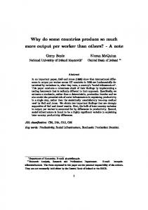
the midst of a financial crunch. Their governments were also better poised to extend unemployment benefits to the jobless during the downturn. By contrast, the shaky fiscal health of the Latin American Two had an opposite effect. They lacked resources to repay their external debt, assist their private sector recovery, and extend unemployment benefits to the unemployed. The contrasting fiscal status of the two groups in the years prior to the emergence of the crisis, from 1991 to 1996, for the East Asian Four, and from 1991 to 2000 for the Latin American Two (1999 for Brazil), is brought out in figures 1 and 2. Government budgets in the East Asian Four during 1991 to 1996 in figure 1 were in surplus in most years whereas they were negative throughout the period from 1991 to 2000 for Argentina, and for Brazil hitting 10 percent of GDP in 1999. Next, high saving rates have a mediating effect on interest rates during a crisis. High overall saving in the economy implies that more domestic funds may be available for lending, and thus for supporting investment even during the crisis phase. Consequently interest rates may shoot up less, and the contraction of investment and GDP in the post-crisis period may be moderated. Thus saving rates in the East Asian Four ranged from over 25 to 35 percent or higher of GDP (figure 3), whereas the saving rate was stagnant at 15 percent for Argentina and declined to that level in 1999 for Brazil from a high of 20 percent in 1991 (figure 4). Finally, a strong export sector would provide the East Asian group with the capability of generating the much- needed foreign exchange in the postcrisis period. Although a few companies went bankrupt because of their inability to repay foreign debt, the survivors benefited from the increased foreign demand resulting from the lower exchange rate. Moreover, companies that were unable to meet their external financial obligations had highly developed manufacturing infrastructure. The depreciated exchange rates made them attractive pickings by foreign investors. These factors contributed to a rapid revival of foreign investor confidence in the East Asian Four. By contrast, the uneven and generally feeble performance of Argentine and Brazilian export sectors was inadequate to bring back foreign creditors, in the process requiring significantly higher interest rates for the purpose. According to the contrasting export performance of the two sets of countries in figure 5, the pre-crisis, average annual growth of Thai exports in dollars was three times that of Argentina in its pre-crisis years. The model, which we present below, is designed to assess the impact of 4
these three macroeconomic features on the interest and exchange rates and therefore on the inflation and GDP growth rates in the post-crisis recovery phase of Argentina in the context of our simulation design.
3
The Model
We begin with the classic Dornbusch (1976) exchange rate over-shooting framework with the three components of the asset market, the money market, and the goods market. The Dornbusch model, however, does not account for investor expectations which are crucial in our framework. The Dornbusch model simply represents the expected depreciation in the exchange rate as a function of its deviation from its equilibrium value. The only shock in the model is a monetary one. Our innovation in the familiar Dornbusch model is precisely in the asset market component. Rather than relying on a monetary shock, we introduce exogenous shocks in the form of investor expectations that affect the economy as it revives from crisis. The expected depreciation of the exchange rate is reconstructed to reflect investor expectations which, in turn, are a function of the three macroeconomic fundamentals mentioned above. We begin with the asset market: The Asset Market rt = r∗ + xt
(1)
xt = θ(et − et ) + (²t + ²)(1 + Φ)
(2)
where Φ represents the macroeconomic fundamental that affects investor expectations. It is defined as: Φ = exp{−χ((tax − g) + z + (1 − γ))} The domestic interest rate, rt , in equation 1 is determined by the world interest rate, r∗ , and the expected rate of exchange rate depreciation, xt . This expected rate of exchange rate depreciation has two components in equation 2. The first component is the difference between the long-run equilibrium exchange rate and the current exchange rate where et is the logarithm of the long-run equilibrium exchange rate, et is the logarithm of the current exchange rate, and θ is an adjustment factor.
5
The second component of the expected exchange rate depreciation, our innovation in the Dornbusch model, is investor expectations. Investor expectations about the depreciation of the exchange rate are based on numerous factors such as the current political and economic climate of a country. For example, if some companies in an emerging market default on their external debt, investors will expect other investors to withdraw their funds from this market. This results in a self-fulfilling speculation against the emerging market currency. In equation 2 of our model, investor speculation against the currency is represented by ²t +², where ²t is a transitory component and ² is a permanent component.5 The more confidence investors have in the macroeconomic fundamentals of the economy, the lower the effect of speculation on the expected depreciation. Φ represents the macroeconomic fundamentals that affect investor expectations in our model. Φ has three components, (tax − g), z, (1 − γ): • (tax − g) represents the pre-crisis government budget balance;6 • z represents the pre-crisis export sector strength. This value is represented by the annual percentage growth of real exports of goods and services relative to the annual percentage growth of real GDP. The growth rates are averaged over three years prior to the onset of the crisis.7,8 ; and 5
The speculation term has transitory and permanent components to account for the fact that a financial crisis occasionally results in permanent GDP decline. Cerra and Saxena (2003) find evidence of permanent losses in GDP levels in the post-crisis phase of East Asian economies. In our model, this implies that long-term GDP is defined as yt = y0 − f (²t + ²). Setting ² = 0, and defining y = yt = y0 , we can also simulate a model without permanent GDP losses. 6 The fiscal data employed in our simulations and their sources are reported in Table 3. For Thailand, the pre-crisis values for government budget balance correspond to 1996 average quarterly real government expenditures less revenues. For Argentina the precrisis values for government budget balance correspond to 1999 average quarterly real government expenditures less revenues. 7 The export and GDP data employed in our simulations and their sources are reported in Table 3. For Thailand, the pre-crisis values for the export sector strength correspond to the annual percentage growth of real exports of goods and services relative to the annual percentage growth of real GDP, averaged over 1994, 1995, and 1996. For Argentina, the pre-crisis values for the export sector strength correspond to the annual percentage growth of real exports of goods and services relative to the annual percentage growth of real GDP, averaged over 1997, 1998, and 1999. 8 A version of the model where export sector strength is modeled as export earnings
6
• (1 − γ) represents the pre-crisis national saving rates.9 The Money Market m − pt = −λrt + φyt
(3)
The money market equilibrium sets money demand, the right-hand side of equation 3, equal to money supply, the left-hand side of equation 3. Here m, pt , and yt are the natural logarithms of nominal money, the price level, and real GDP, respectively. The Goods Market yt = u + δ(et − pt ) + γyt + αg − βtax − σrt p˙ = −π(yt − yt )
(4) (5)
The goods market equilibrium sets aggregate demand, the right-hand side of equation 4, equal to aggregate supply, the left-hand side of equation 4. Here aggregate demand is represented by a shift factor, u (which includes the exogenous and constant demand for exports10 ), the relative price of domestic goods and services, et − pt , income, yt , government expenditures relative to revenue, αg − βtax, and interest rates, rt . The consumers’ marginal propensity to consume in the aggregate demand equation, γ determines the saving rate, 1 − γ. In equation 5, the rate of increase in prices, p, ˙ is proportional to the deviation of GDP, yt , from potential GDP, yt . Equilibrium In equilibrium, the interest rate, GDP and the exchange rate must adjust such that the asset, money, and goods markets are simultaneously in relative to external debt is also analyzed. Our preferred model in which we represent export sector strength via export growth relative to GDP growth gives stronger results than the alternative in which export sector strength is modeled as export earnings relative to external debt. We therefore analyze in depth the results of our preferred model. 9 The saving rate data and their sources are reported in Table 3. For Thailand, the precrisis saving rate corresponds to the 1996 annual saving rate. For Argentina, the pre-crisis saving rate corresponds to the 1999 annual rate. 10 We assume for simplicity that demand for exports is exogenous. The country being modeled is assumed to be a small open economy. We assume that there is always a foreign country that demands its exports. So if the economy produces export goods, these will immediately be purchased by a foreign country.
7
equilibrium. The resulting equilibrium conditions are: yt − yt = −ω(pt − pt )
(6)
et − et = −[(1 − φµδ)/∆](pt − pt )
(7)
p˙ = −πω(pt − pt )
(8)
where, ω = [µ(δ+θσ)+µδθλ] ∆ 1 µ = (1−γ) ∆ = φµ(δ + θσ) + θλ Following rational expectations, the rate at which the current exchange rate adjusts to the long-run equilibrium exchange rate is equal to the rate at which the exchange rates actually adjust. That is, θ = πω.
4
Model Simulations
Initially, we assume that the economy in our model is in equilibrium and investor speculation against the currency is absent. That is, ²0 = ²0 = 0. Then the economy is hit with an external shock such that investors now speculate against the currency. That is ²t > 0, ² > 0. The speculation of investors initially affects the expected exchange rate depreciation, which in turn affects the interest rate. The goods and money markets are affected through the interest rate. The exchange rate, GDP, and prices then adjust accordingly. As time passes, investors speculate less against the currency as the currency adjusts to its new long-run value. Consequently, the speculation of investors against the currency is modeled as an exponentially decreasing shock. ²t = exp{kt}, k < 0, where t represents time.11 The pre-crisis values of the macroeconomic fundamentals affecting investor expectations, Φ, either moderate or amplify the effects of investor speculation. When the macroeconomic fundamental variable is strong, investors have more confidence in the economy, and thus Φ acts to reduce the effects of speculation. The opposite occurs when the macroeconomic fundamental is weak. 11
After the economy is hit with an external shock, the permanent component of the shock, ² ≥ 0, remains constant.
8
As already noted, the purpose of our exercise is to assess the impact of pre-crisis macroeconomic fundamentals on an economy experiencing an exogenous shock that induces investors to speculate against the currency. Having selected a specific macroeconomic fundamental, for example, the government’s pre-crisis fiscal status, we use our model to simulate the Argentine economy in its recovery phase. In the first step, the model simulation is calibrated to approximately match the actual interest rate and exchange rate profiles of Argentina. We refer to this simulation as the base case.12 Next, the Argentine government’s pre-crisis fiscal status is changed to that of Thailand. All other variables and parameters are kept at their base case values. We apply the same shock as the one in the base case. In other words, referring to equation (2),²t and ² remain the same as in the base case. This simulated model is referred to as case 1. Finally, the impact of the pre-crisis government fiscal status is assessed by comparing the case 1 simulation results of the interest rate, the exchange rate, the GDP growth rate, and inflation with the actual values for Thailand. If the case 1 simulated Argentine values are a reasonable match to the actual values for Thailand, then we can suggest that had the pre-crisis fiscal status of Argentina been more like that of Thailand, Argentina’s post-crisis interest rate, exchange rate, GDP growth rate and inflation would have been closer to those of Thailand in the post-crisis period. We repeat these steps in two additional simulations by bringing in export sector strength and saving rate in place of government fiscal status. Thus, in the second simulation, we replace the Argentine pre-crisis export sector strength with that of Thailand. In the third and final simulation. Argentine pre-crisis saving rate is replaced with that of Thailand.
5
The Data
We apply three sets of data in our model: the actual data series for Argentina and Thailand, parameter values, and values of macroeconomic fundamentals. The actual data series include quarterly data of interest rates, exchange rates, GDP, and price levels for each country. Details of these data 12 Our base case simulations of Argentine GDP and inflation track their trends rather than their actual magnitudes.
9
are presented in Table 1. We adopt previously estimated parametric values for our money market and goods market parameters. These estimates and their sources are reported in Table 2. Some of the parameters are calibrated such that the simulated time series of interest rates and exchange rates match the actual data for Argentina and Thailand. For example, ut which represents a shift factor in the aggregate demand equation, is adjusted such that the simulated base case time series match the actual time series for Argentina. Finally, the values of the pre-crisis macroeconomic fundamentals of government expenditures and revenues, export sector strength, and saving rates, and their sources for each country are presented in Table 3. The data in Table 4 below bring out the striking contrast between the crisis impact on the economies of Argentina and Thailand. At its peak, Argentine interest rate at 90.61 percent in 2002,QIII (Table 4, row 3, column 2) was almost six times its level of 15.25 percent in Thailand in 1998, QI and QII (Table 4, row 3, column 3). The high Argentine interest rate reflects the abysmally low investor confidence in its recovery prospects. The difference in crisis severity is also reflected in the exchange rate depreciation. Prior to the crisis, Argentine and Thai exchange rates were fixed to the dollar, the former more strictly than the latter. When they were allowed to float in the post-crisis phase, the peso’s maximum plunge was 258.47 percent in 2002,QIII (Table 4, row 6, column 2) in contrast to the baht’s maximum decline of 82.10 percent in 1998,QI (Table 4, row 6, column 3), almost three times less. The post-crisis GDP growth rates of Argentina and Thailand are also reported in Table 4. The two growth rates are similar in their pattern and magnitude although, at its lowest, Argentina’s GDP growth rate in 2002,QI is slightly more negative at -15.23 percent (Table 4, row 9, column 2) than Thailand’s in 1998,QIII at - 13.92 percent (Table 4, row 9, column 3). Argentina’s GDP growth rate, however, continues to be negative for a longer stretch after the crisis representing a more painful recovery. Finally, inflation soared higher in Argentina than in Thailand in the post-crisis phase. At its height in 2002,QIV the rate was 40.31 percent (Table 4, row 13, column 2) in contrast to Thailand’s 10.35 percent in 1998,QII (row 13, column 3). 10
The combination of high inflation, exchange rate depreciation and soaring interest rate and the persistence of negative GDP growth rate made Argentina’s post-crisis recovery more arduous than for Thailand. Table 4: Actual Rates of Interest, Exchange Rate Depreciation, GDP Growth Rates, and Inflation Rates for Argentina and Thailand 1
1 2 3 4
Variable* Pre-crisis interest rate Maximum post-crisis interest rate Equilibrium post-crisis interest rate Pre-crisis exchange rate depreciation Maximum post-crisis depreciation Equilibrium post-crisis depreciation Pre-crisis GDP growth rate Maximum negative post-crisis GDP growth rate Maximum positive post-crisis GDP growth rate Equilibrium post-crisis GDP growth rate
5 6 7 8 9 10 11 12 Pre-crisis inflation rate 13 Maximum post-crisis inflation rate 14 Equilibrium post-crisis inflation rate
2
3
4
Actual Value for Argentina
Actual Value for Thailand
Difference
9.66% 90.61% 13.90%
13% 15.25% 6.50%
-3.34% 75.36% 7.40%
0.00% 258.47% -20.91%
2.40% 82.10% -2.16%
-2.40% 176.37% -18.75%
-0.33% -15.23% 8.62% 8.62%
1.00% -13.92% 8.41% 6.73%
-1.33% -1.31% 0.21% 1.89%
-0.78% 40.31% 5.20%
4.37% 10.35% 1.97%
-5.15% 29.96% 3.24%
Notes: ∗ All variables are measured on a quarterly basis. 1. The pre-crisis rates of all variables refer to their values in the quarter preceding 2000,QIV for Argentina and 1997,QII for Thailand. 2. The maximum post-crisis rates represent the highest values of the variables in the post-crisis period. 3. The equilibrium post-crisis rates represent their final and stable values in the post-crisis period after all factors have fully adjusted in the simulation. The actual equilibrium values refer to 2003,QIII for Argentina (this was the most recent value available at the time this analysis was done) and 2003,QI for Thailand. 4. The Argentine peso was allowed to float in 2002,QI. The baht was allowed to float in 1997,QIII.
11
6
Simulation Results
In our simulations, the adoption of Thailand’s pre-crisis macroeconomic fundamentals for Argentina should result in an easier recovery path for Argentina, resembling that in Thailand, in terms of interest rate, exchange rate depreciation, GDP growth, and inflation. Recall that our base case simulates the Argentine economy from 2000,QIII to 2003,QIII. Each version of the model alters the base case simulation by changing the value of a pre-crisis macroeconomic fundamental from its Argentine value to its Thai value. The resulting simulation is compared to the actual performance of the recovering Thai economy. A closer match brings out the effectiveness of the particular pre-crisis macroeconomic fundamental. The simulation results are summarized in Tables 4.1- 4.4, one each for interest rate, exchange rate depreciation, GDP growth rate and inflation rate, and presented in figures 6-9. We notice similar patterns in these variables across the simulations: interest rates shoot up, exchange rates decline, GDP growth rates tumble, and inflation rates go up after the shock and subsequently adjust to take their equilibrium values. However, the simulation version with the pre-crisis export sector strength gives significantly lower values of interest rate, exchange rate depreciation, GDP growth rate decline and inflation rate than the alternatives. This version outperforms the simulations in which the pre-crisis macroeconomic fundamentals represent the government’s fiscal status and the economy’s saving rate. We discuss the details of our simulations below beginning with interest rates.
6.1
Interest Rates
In figure 6, the base case simulation tracks the actual Argentine interest rate relatively well. The maximum post-crisis interest rate for Argentina was 90.61 percent (Table 4.1, row 2, column 3). The base case simulation, emulating the Argentine economy, attains a similar maximum post-crisis interest rate of 90.37 percent (Table 4.1, row 5, column 3). In contrast, the actual Thai maximum post-crisis interest rate, 15.25 percent (Table 4.1, row 4, column 3) was 75.36 basis points lower than the corresponding Argentine rate. When Argentina’s pre-crisis fiscal status is changed to that of Thailand, the maximum Argentine post-crisis interest rate drops by only 0.22 basis points (Table 4.1, row 8, column 3). By contrast, if the pre-crisis govern12
ment fiscal status played a critical role in post-crisis recovery, the maximum post-crisis interest rate in the simulation would have dropped by a number closer to 75.36 basis points (the difference between the actual Argentine and Thai interest rates, Table 4.1, row 4, column 3). Despite a robust, pre-crisis fiscal status closer to Thailand’s, the crisis would have landed Argentina in exorbitant interest rates. However the imposition of the Thai export sector strength to pre-crisis Argentina, the maximum post-crisis interest rate in Argentina is reduced by 45.43 basis points (Table 4.1, row 11, column 3). In figure 6, this version brings the simulated value of Argentine interest rate remarkably close to the actual Thai value in contrast to the simulation versions employing Thailand’s pre-crisis fiscal status and saving rate (to be analyzed below). If Argentina had the pre-crisis export sector strength of Thailand, its interest rate would not have soared to 90 percent. It would have capped around a more manageable 45 percent. Finally, the augmentation of the pre-crisis saving rate of Argentina to that of Thailand pulls down the maximum post-crisis interest rate of the simulated Argentine economy by a miniscule 0.31 basis points (Table 4.1, row 14, column 3). The post-crisis interest rate in Argentina turns out to be insensitive to the pre-crisis saving rate.
13
Table 4.1: Interest Rate Analysis 1
1 2 3 4 5 6 7 8 9 10 11 12 13 14
2
3
4
Maximum Post- Equilibrium Pre-Crisis Crisis Interest Post-Crisis Interest Rate Rate Interest Rate
Variable* 9.66% 90.61% Actual value for Argentina 13% 15.25% Actual value for Thailand -3.34% 75.36% Difference 8.00% 90.37% Base case ** Scenario 1 - Replace Argentine fiscal status with that of Thailand 8.00% 90.15% Case 1*** 0.00% 0.22% Difference = base case - case 1
12.37% 0.01%
Scenario 2 - Replace Argentine export sector strength with that of Thailand 8.00% 44.94% 9.97% Case 1 *** 0.00% 45.43% 2.41% Difference = base case - case 1 Scenario 3 - Replace Argentine saving rate with that of Thailand 8.00% 90.06% Case 1*** 0.00% 0.31% Difference = base case - case 1
Notes: ∗ All variables are measured on a quarterly basis. ∗∗ Base case values refer to simulated Argentine values. ∗∗∗ Case1 values are simulated Argentine values which result when its pre-crisis macroeconomic fundamental is replaced with a pre-crisis Thai value. 1. The pre-crisis rates prevailed in the quarter preceding 2000,QIV for Argentina and 1997,QII for Thailand. 2. The maximum post-crisis rates represent their highest values in the post-crisis period. 3. The equilibrium post-crisis rates represent their final and stable values in the post-crisis period after all factors have fully adjusted in the simulation. These actual values are 2003,QIII value for Argentina (this was the most recent value available at the time this analysis was done) and 2003,QI value for Thailand. 4. GDP growth simulations assume a relatively stable GDP level with a zero GDP growth rate for the quarter prior to crisis onset. 5. The Argentine peso was allowed to float in 2002,QI, the baht in 1997,QIII. These notes apply to Tables 4.2-4.4 as well.
6.2
13.90% 6.50% 7.40% 12.38%
Exchange Rate Depreciation
The maximum depreciation of the actual Argentine exchange rate was 258.47 percent in 2002,QIII, (Table 4.2, row 2, column 3). The exchange rate in our base case simulation attains a maximum depreciation of 216.71 percent (Table 4.2, row 5, column 3). By contrast, the maximum post-crisis depreciation of the Thai baht was relatively modest at 82.10 percent (Table 14
12.37% 0.01%
4.2, row 3, column 3), 176.3 percent lower than the peso. Figure 7 brings out this striking contrast. As with the interest rate, the peso exchange rate is relatively insensitive to Argentine government’s pre-crisis fiscal status. When it is replaced by the pre-crisis fiscal status of Thailand, the maximum depreciation of the peso is reduced by only 0.98 percent (Table 4.2, row 8, column 3). If the government’s pre-crisis fiscal status were a critical factor in affecting its level, the massive actual decline of the peso, post-shock, would have been reduced substantially by 176.37 percent reaching the baht’s post-crisis maximum decline of 82.10 percent (Table 4.2, row 4, column 3). By contrast, a change in the pre-crisis export sector strength of Argentina to that of Thailand significantly reduces the peso’s depreciation in the post-crisis period in Figure 7. The maximum depreciation is reduced by as much as 148.88 percent (Table 4.2, row 11, column 3), closer to the 176.37 percent difference between the actual peso-baht maximum tumble (Table 4.2, row 4, column 3). Finally, the impact of the pre-crisis saving rate on the post-crisis peso exchange rate decline is similar to the impact of the pre-crisis fiscal status of the government: the peso’s depreciation is insensitive to the pre-crisis saving rate in the simulation. The maximum post-crisis depreciation of the peso is contained by only 5.39 percent (Table 4.2, row 14, column 3). The simulation results suggest a substantially moderate post-shock interest and exchange rate movements associated with a strong pre-crisis export sector strength. As a result, Argentina’s recovery path could possibly have been less prolonged and painful.
6.3
GDP Growth Rates
As noted earlier, our base case simulations understate the magnitudes of Argentina’s GDP growth and inflation rates while tracking their trends. In figure 8, during the post-crisis period, actual GDP in Argentina and Thailand experience a significant decline, with negative growth rates, in the initial post-crisis quarters. As the economies recover, both GDP move up. Thus the actual GDP growth rates of the two economies follow a similar 15
Table 4.2: Exchange Rate Depreciation Analysis 1
1 2 3 4 5 6 7 8 9 10 11 12 13 14
2
3
4
Maximum Post- Equilibrium Post-Crisis Crisis Pre-Crisis Depreciation of Depreciation of Depreciation Exchange Rate Exchange Rate
Variable* 0.00% 258.47% Actual value for Argentina 2.40% 82.10% Actual value for Thailand -2.40% 176.37% Difference 0.00% 216.71% Base case ** Scenario 1 - Replace Argentine fiscal status with that of Thailand 0.00% 215.73% Case 1 *** 0.00% 0.98% Difference = base case - case 1
-20.91% -2.16% -18.75% 0.00% 0.00% 0.00%
Scenario 2 - Replace Argentine export sector strength with that of Thailand 0.00% 67.83% 0.00% Case 1*** 0.00% 148.88% 0.00% Difference = base case - case 1 Scenario 3 - Replace Argentine saving rate with that of Thailand 0.00% 211.32% Case 1*** 0.00% 5.39% Difference = base case - case 1
path. The maximum negative post-crisis actual GDP growth of Argentina is only 1.31 percent lower than that of Thailand (Table 4.3, row 4, column 3). Our simulations suggest that if Argentina had the pre-crisis fiscal status of Thailand, its maximum negative GDP growth would have matched it in the base case simulation in which Argentina retains its own pre-crisis fiscal status (Table 4.3, row 8, column 3). Essentially, the pre-crisis fiscal status has no effect on Argentine GDP growth as it recovers. Similarly, the post-crisis Argentine economy is insensitive to the pre-crisis saving rate. Changing the pre-crisis saving rate of Argentina to that of Thailand results in zero change in the post-crisis GDP growth path (Table 4.3, row 14, column 3, also figure 8). However, when we replace the pre-crisis export sector strength of Argentina with that of Thailand in our simulated Argentine economy, Argentina’s maximum negative GDP growth rate is pulled up by 0.19 percent (Table 4.3, row 11, column 3). The actual maximum negative post-crisis
16
0.00% 0.00%
GDP growth of Argentina is 1.31 lower than in Thailand (Table 4.3, row 4, column 3). In figure 8, the attribution of the pre-crisis export sector strength of Thailand to Argentina is most effective in reducing fluctuations in GDP growth rate in recovering Argentina. Table 4.3: GDP Growth Rate Analysis 1
1 2 3 4 5 6 7 8 9 10 11 12 13 14
2
3
4
5
Maximum Maximum Positive Pre-Crisis Negative Post-Crisis Equilibrium GDP Post-Crisis GDP Post-Crisis Growth GDP Growth Growth GDP Growth
Variable* -0.33% -15.23% Actual value for Argentina 1.00% -13.92% Actual value for Thailand -1.33% -1.31% Difference 0.00% -1.25% Base case ** Scenario 1 - Replace Argentine fiscal status with that of Thailand 0.00% -1.25% Case 1*** 0.00% 0.00% Difference = Base case - case 1
8.62% 8.41% 0.21% 0.47%
8.62% 6.73% 1.89% 0.00%
0.47% 0.00%
0.00% 0.00%
Scenario 2 - Replace Argentine export sector strength with that of Thailand 0.00% -1.06% 0.43% Case 1*** 0.00% -0.19% 0.04% Difference = Base case - case 1
0.00% 0.00%
Scenario 3 - Replace Argentine saving rate with that of Thailand 0.00% -1.25% Case 1*** 0.00% 0.00% Difference = Base case - case 1
0.00% 0.00%
6.4
0.47% 0.00%
Inflation
The maximum post-crisis inflation rate in Thailand is 29.96 percent lower than in Argentina (Table 4.4, row 4, column 3). As before, the potentially large impact of a pre-crisis macroeconomic fundamental in mediating investor expectations, and thus reducing the severity of the crisis, would result in a significant reduction of the inflation rate in recovering Argentina if its pre-crisis macroeconomic fundamentals were to assume Thai values. In our simulations, Argentina’s assumption of Thai fiscal status and saving rate lowers the maximum post-crisis inflation rate of Argentina by a
17
mere 0.01 percent in both cases (Table 4.4, row 8, column 3 and Table 4.4, row 14, column 3). The Argentine inflation rate is insensitive to its pre-crisis fiscal status and saving rate. By contrast, Argentina’s maximum inflation rate in the recovery phase drops by 1.88 percent when it takes the pre-crisis export sector strength of Thailand (Table 4.4, row 11, column 3). Table 4.4: Inflation Rate Analysis 1
1 2 3 4 5 6 7 8 9 10 11 12 13 14
7
2
3
Maximum Pre-Crisis Post-Crisis Inflation Rate Inflation Rate
4 Equilibrium Post-Crisis Inflation Rate
Variable* -0.78% 40.31% Actual value for Argentina 4.37% 10.35% Actual value for Thailand -5.15% 29.96% Difference 0.00% 4.32% Base case** Scenario 1 - Replace Argentine fiscal status with that of Thailand 0.00% 4.32% Case 1 *** 0.00% 0.01% Difference = Base case - case 1
5.20% 1.97% 3.24% 0.00% 0.00% 0.00%
Scenario 2 - Replace Argentine export sector strength with that of Thailand 0.00% 2.44% 0.00% Case 1 *** 0.00% 1.88% 0.00% Difference = Base case - case 1 Scenario 3 - Replace Argentine saving rate with that of Thailand 0.00% 4.31% Case 1 *** 0.00% 0.01% Difference = Base case - case 1
Conclusions
We analyze the post-crisis performance of two crisis-affected economies, Argentina and Thailand, with vastly different pre-crisis macroeconomic fundamentals by applying a simple macroeconomic model. Their pre-crisis macroeconomic fundamentals, among them their governments’ fiscal status, the national saving rates, and export sector strength, can be expected to affect post-crisis recovery differently. In fact, our model simulations suggest that the pre-crisis difference in export sector strength between Argentina and Thailand (acting through investor expectations) is large enough to explain most of the difference in post-crisis interest rate and exchange rate 18
0.00% 0.00%
movements between the two countries. The GDP growth and inflation rate results are quantitatively less strong; however, the pre-crisis difference in export sector strength is able to explain some of the post-crisis difference in these two variables as well. In other words, if Argentina had the pre-crisis export sector strength of Thailand, Argentina’s post-crisis recovery path could have been closer to that of Thailand. On the other hand, a strong fiscal status and a high national saving rate in the pre-crisis years could not have spared the Argentine economy from high interest rates and substantial peso depreciation leading in turn to substantial GDP decline and high inflation. The export earning capacity of an economy reflects its debt repayment potential by generating foreign exchange earnings and restoring investor confidence. The contrasting results suggest that investors focus essentially on an economy’s ability to generate foreign exchange and repay its external debts. However, our model lacks microeconomic foundations that could adequately capture the interaction among consumers, producers, foreign investors and the government. We plan to design and empirically test such a model with appropriate microeconomic underpinning. Despite this shortcoming, we believe that our simulation results linking superior post-crisis recovery to pre-crisis export strength are eminently credible.
19
8
Appendix: Derivation of Model
The model is defined by the following five equations: Asset Market rt = r∗ + xt
(1)
xt = θ(et − et ) + (²t + ²)(1 + Φ)
(2)
φ = exp{−χ((tax − g) + z + (1 − γ))} Money Market m − pt = −λrt + φyt
(3)
yt = u + δ(et − pt ) + γyt + αg − βtax − σrt
(4)
The Goods Market
p˙ = −π(yt − yt )
(5)
We take as given (i.e., exogenous) values for all parameters and m, r∗ , g, tax, (²t + ²), yt . Step 1: Goods and Asset Market Equilibrium For a given shock, (²t + ²), the economy converges to equilibrium where: yt = yt , et = et , pt = pt =⇒ r = r∗ + (² + ²)(1 + Φ) Substituting equations (1) and (2) into equation (4), we get the equilibrium value for yt : yt = µ[u + δ(et − pt ) + αg − βtax − σr∗ − σ(²t + ²)(1 + Φ)] 1 µ = 1−γ
(6)
Subtracting equation (6) from (4), we get yt − yt = µ[(δ + σθ)(et − et ) − µδ(pt − pt )]
(7)
Step 2: Money and Asset Market Equilibrium For a given shock, (²t + ²), the economy converges to equilibrium where: yt = yt , et = et , pt = pt =⇒ r = r∗ + (² + ²)(1 + Φ) Substituting equations (1) and (2) into equation (3), we get pt = m + λr∗ + λθ(et − et ) + λ(²t + ²)(1 + Φ) − φyt 20
(8)
The equilibrium value for pt in (8) is given by pt = m + λr∗ + λ(²t + ²)(1 + Φ) − φyt
(9)
Subtracting equation (9) from (8), we get pt − pt = λθ(et − et ) − φ(yt − yt )
(10)
Step 3: Combining Goods, Asset, and Money Market Equilibrium Substituting (et − et ) from equation (10) into equation (7), we derive (yt − yt ) = −ω(pt − pt )
(11)
ω = [µ(δ + θσ) + µδθλ]/∆ ∆ = φµ(δ + θσ) + θλ Rational Expectations dictate that θ = πω Substituting equation (11) into equation (10), we derive et − et = −
(1 − φµδ) (pt − pt ) φµ(δ + σθ) + λθ
(12)
Substituting (11) into (5), we get p˙ = −πω(pt − pt )
(13)
Step 4: Defining equilibrium exchange rate and prices From equation (9), we have pt = m + λr∗ + λ(²t + ²)(1 + Φ) − φyt
(14)
Substituting equation (6) into (9), we get et =
[(1 − µδφ)yt − µu + µδm + µ(δλ + σ)r∗ ] µδ [µ(δλ + σ)(²t + ²)(1 + Φ) − µαg + µβtax] + µδ
Step 5: Solving for all the variables We take as given (i.e., exogenous) values for m, r∗ , g, tax, (²t + ²), yt . Substituting these values into equations (14) and (15), we have m, r∗ , g, tax, (²t + ²), yt =⇒ pt , et We can then solve for the differential equation from (13): 21
(15)
pt , p˙t =⇒ pt Using equation (11), we can solve for yt pt , pt =⇒ yt Using equation (12), we can solve for et pt , et , pt =⇒ et Using equations (1) and (2), we can solve for rt r∗ , et , et , (²t + ²) =⇒ rt Step 6: Simulation 1. Initially we assume ²0 = ²0 = 0 and we have m, r∗ , y0 . Applying Step 5, we solve for the initial values of all the variables; 2. A shock hits the economy: ²t = exp{kt}, k < 0, ²t ≥ 0; 3. We define yt = y0 − f (²t + ²). Therefore, for each time, t, ²t =⇒ yt . 4. Next, for each time, t, we have m, r∗ , (²t + ²), yt . Applying Step 5, we solve for the time, t, values of all the variables. . 5. We repeat parts 3 and 4 of the simulation process until, ²t = 0, thereby reaching the long-run equilibrium. The permanent component of the shock has permanently reduced the equilibrium value of yt , permanently depreciated et , and permanently increased the price level pt . 6. In our simulations, we define the base case as the scenario in which the values of Φ, the macroeconomic fundamental that affects investor expectations, reflect the Argentine values of fiscal status, export sector strength, and saving rate1 [(tax−g), z, (1−γ)]. In the alternative cases, the simulation described above is performed by changing the value of one macroeconomic fundamental; for example z, is changed to its Thai value.2 1
Argentina: The pre-crisis fiscal status is measured as the 1999 average quarterly government expenditures less revenue. The pre-crisis export sector strength is measured as the average 1997-99 annual percentage growth of real exports divided by the annual percentage growth of real GDP. The pre-crisis saving rate is measured as the 1999 annual saving rate. Details are given in Table 2. 2 Thailand : The pre-crisis fiscal status is measured as the 1996 average quarterly government expenditures less revenue. The pre-crisis export sector strength is measured as the average 1994-96 annual percentage growth of real exports divided by the annual percentage growth of real GDP. The pre-crisis saving rate is measured as the 1996 annual saving rate. Details are given in Table 2.
22
References [1] Baharumshah, Ahmad Z., Marwan A. Thanoon and Salim Rashid. 2003. “Savings Dynamics in the Asian Countries.” Journal of Asian Economics. vol. 13, pp.827-845. [2] Caballero, Ricardo J. and Arvind Krishnamurthy. 2001. “A ”Vertical” Analysis of Crises and Intervention: Fear of Floating and Ex-ante Problems” NBER Working Paper No.8428. [3] Calvo, Guillermo A. 2003. “Explaining Sudden Stops, Growth Collapse and BOP Crises: The Case of Distortionary Output Taxes.” NBER Working Paper No.9864. [4] Calvo, Guillermo A. 1998. “Capital Flows and Capital-Market Crises: The Simple Economics of Sudden Stops” Journal of Applied Economics. vol.1, No.1, pp.35-54. [5] Calvo, Guillermo A. and Frederic S. Mishkin. 2003. “The Mirage of Exchange Rate Regimes for Emerging Market Countries.” NBER Working Paper No.9808. [6] Calvo, Guillermo A. and Carmen M. Reinhart. 2000. “When Capital Inflows Come to a Sudden Stop: Consequences and Policy Options” in Key Issues in Reform of the International Monetary and Financial System, Peter Kenen and Alexandre Swoboda, eds. International Monetary Fund, Washington,DC. [7] Cerra, Valerie and Sweta C. Saxena. 2003. “Did Output Recover from the Asian Crisis?” IMF Working Paper 03/48. [8] Cespedes, Luis F., Roberto Chang, and Andres Velasco. 2000. “Balance Sheets and Exchange Rate Policy.” NBER Working Paper No.7840. [9] Charoenseang, June and Pornkamol Manakit. 2002. “Financial Crisis and Restructuring in Thailand.” Journal of Asian Economics. vol. 13, pp.597-613. [10] Chowdhury, Abdur R. 1997. “The Financial Structure and the Demand for Money in Thailand.” Applied Economics. vol. 29, pp.401-409. [11] Christiano, Lawrence J., Christopher Gust and Jorge Roldos. 2003. “Monetary Policy in a Financial Crisis.” Journal of Economic Theory. July. 23
[12] Claessens, Stijn, Daniela Klingebiel and Luc Laeven. 2001. “Financial Restructuring in Systemic Crises: What Policies to Pursue?” NBER Conference on Management of Currency Crises, Monterey, March 2831, 2001. [13] Corsetti, Giancarlo, Paolo Pesenti and Nouriel Roubini. 2001. “Fundamental Determinants of the Asian Crisis: The Role of Financial Fragility and External Imbalances” in Regional and Global Capital Flows: Macroeconomic Causes and Consequences, Ito, Takatoshi and Anne O. Krueger, eds. National Bureau of Economic Research-East Asia Seminar on Economics. [14] Dekle, Robert and Mahmood Pradhan. 1999. “Financial Liberalization and Money Demand in the ASEAN Countries.” International Journal of Finance and Economics. vol. 4, pp.205-215. [15] Desai, Padma. 2003. “Explorations in Light of Financial Turbulence from Asia to Argentina.” Conference on the Future of Globalization: Explorations in Light of Recent Turbulence, Yale Center for the Study of Globalization, Yale University, October 10-11. [16] Desai, Padma. 2003. Financial Crisis, Contagion, and Containment: From Asia to Argentina New Jersey: Princeton University Press. [17] Dornbusch, Rudiger. 1976. “Expectations and Exchange Rate Dynamics.” Journal of Political Economy. vol. 84 (6), pp.1161-1176. [18] Ghosh, Atish and Paul R. Masson. 1991. “Model Uncertainty, Learning and the Gains from Coordination.” American Economic Review. vol. 81 (3), pp.465-479. [19] Kaminsky, Graciella L. and Carmen M. Reinhart. 1999. “The Twin Crises: The Causes of Banking and Balance-of-Payments Problems.” American Economic Review. vol. 89(3), pp.473-500. [20] Kaminsky, Graciella L. ,Carmen M. Reinhart, and Carlos A. Vegh. 2003. “The Unholy Trinity of Financial Contagion.” NBER Working Paper No.10061. [21] Koo, Jahyeong and Sherry L. Kiser. 2001. “Recovery from a Financial Crisis: The Case of South Korea.” Economic and Financial Policy Review, Federal Reserve Bank of Dallas, vol.4, pp. 24-36.
24
[22] Krugman, Paul. 1999. The Return of Depression Economics. New York: WW Norton & Company. [23] Lahiri, Amartya and Carlos A. Vegh. 2001. ”Living with the Fear of Floating: An Optimal Policy Persepective” NBER Working Paper No.8391. [24] Park, Yung C. and Jong W. Lee. 2001. “Recovery and Sustainability in East Asia” Conference on Management of Currency Crises, NBER, March 28-31. [25] Rodrik, Dani and Andres Velasco. 1999. “Short-Term Capital Flows” NBER Working Paper No.7364.
25
Tables and Figures Table 1: Actual Series Series Thailand
Symbol
Real GDP Lending interest rate (%)
Y
Source
Frequency
Year(s)
Quarterly
1997,QI-2003,QI
p&
Economist Intelligence Unit Country Data Economist Intelligence Unit Country Data
Quarterly
1997,QI-2003,QI
Consumer prices (% average change per annum) r
Economist Intelligence Unit Country Data
Quarterly
1997,QI-2003,QI
Economist Intelligence Unit Country Data
Quarterly
1997,QI-2003,QI
Exchange rate Baht:US$ (period average) Argentina
E
Quarterly
2000,QIII-2003,QIII
p&
Economist Intelligence Unit Country Data Economist Intelligence Unit Country Data
Quarterly
2000,QIII-2003,QIII
Consumer prices (% average change per annum) r
Economist Intelligence Unit Country Data
Quarterly
2000,QIII-2003,QIII
Exchange rate Peso:US$ (period average)
Economist Intelligence Unit Country Data
Quarterly
2000,QIII-2003,QIII
Real GDP Lending interest rate (%)
Y
E
26
Table 2: Parameter Estimates Table 2A: Goods Market Parameter
Value
Interpretation Sensitivity of aggregate demand to relative 0.11 prices of domestic goods and services Proportion of income spent on purchases of goods and services (approximately the 0.85 inverse of the saving rate) Proportion of income spent on purchases of goods and services (approximately the 0.7 inverse of the saving rate) Sensitivity of aggregate demand to interest 0.15 rates Sensitivity of aggregate demand to 0.3 government expenditures
δ γArgentina γ Thailand σ α β
0.2 Sensitivity of aggregate demand to taxes Proportion representing the constant relationship between changes in output and 0.2 changes in prices
π u
1.472 Shift parameter
y Argentina
69 billion pesos Initial long-run equilibrium output
y Thailand
779 billion bahts Initial long-run equilibrium output
Source of Estimate Ghosh and Masson (1991)
World Development Indicators World Development Indicators, Baharumshah, Thanoon, and Rashid (2003) Ghosh and Masson (1991) Calibrated* Calibrated*
Calibrated* Calibrated* Economist Intelligence Unit Country Data, Quarterly Real GDP 2000 average Economist Intelligence Unit Country Data, Quarterly Real GDP 1996 average
*These parameter values are adjusted so that the simulated Argentine time series match the actual Argentine time series.
Table 2B: Money Market Parameter
φ λ MThailand
MArgentina
Value
Interpretation Sensitivity of real money demand to real 1 income Sensitivity of real money demand to interest 0.04 rates
Source of Estimate Chowdhury (1997), Dekle and Pradhan (1999) Dekle and Pradhan (1999)
3726 billion bahts Money Supply
Economist Intelligence Unit Country Data, M2 Money Supply, 1996,QIV
91 billion pesos Money Supply
Economist Intelligence Unit Country Data, M2 Money Supply, 2000,QIV
27
Table 2C: Asset Market Parameter
Value
Interpretation
8% World interest rate Factor for adjustment of current exchange 0.2447 rate to long-run exchange rate value Sensitivity of investor speculation to pre0.033 crisis macroeconomic fundamental
r*
θ χ
Source of Estimate World Development Indicators, approximated by the average of 19952000 US prime rate Endogenously Determined** Calibrated*
*These parameter values are adjusted so that the simulated Argentine time series match the actual Argentine time series. **This parameter value is determined endogenously within the model (refer to p.8 of the text).
Table 2D: Shock Equation Parameter
κ
ε ε0
Value
Interpretation
Source of Estimate
-0.07 Shock propagation factor 0.01 Permanent component of shock
Calibrated* Calibrated*
0.178 Initial value of transitory component of shock Calibrated*
*These parameter values are adjusted so that the simulated Argentine time series match the actual Argentine time series.
28
Table 3: Macroeconomic Fundamentals Variable
Value
Interpretation
GArgentina
15 billion pesos
Government expenditures, quarterly data
Source of Estimate Economist Intelligence Unit Country Data, Quarterly Real Government Expenditures, 1999 average
Government expenditures, quarterly data
Economist Intelligence Unit Country Data, Quarterly Real Government Expenditures, 1996 average
Government revenues, quarterly data
Economist Intelligence Unit Country Data, Quarterly Real Government Expenditures, 1999 average
Government revenues, quarterly data
Economist Intelligence Unit Country Data, Quarterly Real Government Expenditures, 1996 average
GThailand
TArgentina
TThailand
ZArgentina
ZThailand
ZArgentina
ZThailand
1−γArgentina 1−γ Thailand
137 billion bahts
14 billion pesos
142 billion bahts
4.02/-0.11 = Annual percentage growth of real exports of goods and services/ annual percentage growth of real GDP. Averaged over 3 years prior to the crisis -36.55 (1997,1998,1999) 8.06/8.04 = Annual percentage growth of real exports of goods and services/ annual percentage growth of real GDP. Averaged over 3 years prior to the crisis 1.00 (1994,1995,1996)
World Development Indicators
World Development Indicators 1/Total debt service (% exports of goods and services) = Exports of goods and services/Total debt payment. Averaged over 3 years 1.50 prior to the crisis. World Development Indicators 1/Total debt service (% exports of goods and services) = Exports of goods and services/Total debt payment. Averaged over 3 years World Development Indicators 8.00 prior to the crisis. Saving Rate = 1-Proportion of income spent on purchases of 0.15 goods and services (1999) World Development Indicators Saving Rate = 1- Proportion of World Development Indicators, income spent on purchases of Baharumshah, Thanoon, and Rashid (2003) 0.30 goods and services (1996)
29
30
Budget Surplus as a Percentage of GDP
-4
-3
-2
-1
0
1
2
3
4
5
6
1990
1991
1992
1994
Korea
Source : Economist Intelligence Unit.
Years
1993
Indonesia
Figure 1: Government Budget Balance of East Asian Countries
1995
Malaysia
1996
Thailand
31
Budget Surplus as a Percentage of GDP
-12
-10
-8
-6
-4
-2
0
1990
1991
Argentina
1992
1994
Years
1995
1996
1997
1998
Source : Economist Intelligence Unit. Data prior to 1994 for Argentina and prior to 1995 for Brazil are not available.
1993
Brazil
Figure 2: Government Budget Balance of Argentina and Brazil
1999
2000
32
National Saving as a Percentage of GDP
0
5
10
15
20
25
30
35
40
1990
1991
Year
1993
1994
Korea
1995
Malaysia
Source: Economist Intelligence Unit. Aggregate national saving by the public and private sectors as a percent of nominal GDP.
1992
Indonesia
Figure 3: Saving Rates of East Asia Countries
1996
Thailand
33
National Saving as a Percentage of GDP
0
5
10
15
20
25
1990
1991
1993
1994
Years
1995
1996
1997
1998
Argentina
Source: Economist Intelligence Unit. Aggregate national saving by the public and private sectors as a percent of nominal GDP.
1992
Figure 4: Saving Rates of Argentina and Brazil
1999
2000
Brazil
34
U.S. Dollars (billions)
$0
$20
$40
$60
$80
$100
$120
$140
$160
$180
$200 Brazil
Indonesia
Korea
Malaysia
Thailand
Source: Economist Intelligence Unit.
Years
1980 1981 1982 1983 1984 1985 1986 1987 1988 1989 1990 1991 1992 1993 1994 1995 1996 1997 1998 1999 2000 2001 2002 2003
Average Annual Export Growth Rate 1980-1999 Argentina 6.5% Brazil 5.3% 1980-1996 Indonesia 5.9% Korea 13.8% Malaysia 12.6% Thailand 15.1%
Argentina
Figure 5: Total Annual Exports (f.o.b.) in U.S. Dollars
35 0
10
20
30
40
50
60
70
80
90
100
0
5
10
Quarters After Shock
15
20
Argentina’s Actual Interest Rate Simulation: Base Case Simulation: Argentina with Thai Fiscal Status Simulation: Argentina with Thai Export Sector Strength Simulation: Argentina with Thai Saving Rate Thailand’s Actual Interest Rate
Figure 6: Interest Rate Response to Shock
25
Source: The actual interest rates for Thailand and Argentina are lending rates put together from the Economist Intelligence Unit (EIU); EIU Source: IMF, International Financial Statistics.
Interest Rates (%)
Figure 6: Interest Rate Response to Shock Notes: 1. The financial crisis began in Argentina in the fourth quarter of 2000 (2000,QIV) and hit Thailand in the second quarter of 1997 (1997,QII). In the figure, the quarter preceding the shock (Q0) corresponds to 2000,QIII for Argentina, and 1997,QI for Thailand; 2. The interest rate paths generated by the three simulations of the base case, next, of Argentina with Thai fiscal status, and finally, of Argentina with Thai saving rate almost perfectly overlap, creating only one visible solid line in the figure. Recall that the base case represents Argentine values generated by our model. This overlap reflects the weakness of the pre-crisis fiscal status and saving rate in affecting the post-crisis interest rate. In other words, even if Argentina had the pre-crisis fiscal status or saving rate of Thailand, the post-crisis interest rate of Argentina would match that in the base case in which Argentina retains its own pre-crisis fiscal status and saving rate; 3. The interest rate path generated by the simulation of Argentina with Thai export strength produces post-crisis interest rates that are significantly lower than those resulting from the base case simulation. In the context of our model, this result implies that the post-crisis interest rates in Argentina would have been much lower, closer to the post-crisis interest rates of Thailand if Argentina had the pre-crisis export sector strength of Thailand; 4. We undertake the following steps for deriving the interest rates in the figure. Solving the differential equation for prices (equation 8, p.7), we obtain the path of prices in the quarters after the shock. Substituting prices in equations 6 and 7 (p.7), we solve for GDP and the exchange rate, respectively. Substituting the exchange rate in equations 1 and 2 (p.5), we obtain the interest rates. Details of the calculations for solving each series are in the Appendix. The solutions are generated in Matlab.
36
37
Depreciation (% change per annum)
−50
0
50
100
150
200
250
300
0
10
15
Quarters After Exchange Rate Depreciation
20
Source: Actual baht and peso exchange rates are from Economist Intelligence Unit (EIU); EIU Source: IMF, International Financial Statistics.
5
Argentina’s Actual Exchange Rate Depreciation (Peso/USD,quarterly) Simulation: Base Case Simulation: Argentina with Thai Fiscal Status Simulation: Argentina with Thai Export Sector Strength Simulation: Argentina with Thai Saving Rate Thailand’s Actual Exchange Rate Depreciation (Baht/USD,quarterly)
Figure 7 : Depreciation of Exchange Rates in Response to Shock
25
Figure 7: Exchange Rate Depreciation in Response to Shock Notes: 1. In the years preceding the onset of the crisis and for some time after that, the Argentine peso and the Thai baht were pegged to the U.S. dollar, the former under a regime resembling a currency board, and the latter under a managed exchange rate arrangement. The peso was allowed to float in 2002,QI, and the baht in 1997,QIII. In the figure, Q0 corresponds to the quarter preceding the currency float–2001,QIV for Argentina and 1997,QII for Thailand; 2. The depreciation path generated by the simulations of the base case, and of Argentina with Thai fiscal status almost perfectly overlap, creating only one visible solid line in the figure. This result reflects the weakness of the fiscal status in affecting post-crisis exchange rate depreciation. Even if Argentina had the pre-crisis robust fiscal status of Thailand, the post-crisis exchange rate depreciation of Argentina would remain the same as in the base case in which Argentina retains its own pre-crisis weak fiscal status; 3. The exchange rate depreciation path generated by the simulation of Argentina with Thai saving rate is only slightly lower than the base case simulation path. In other words, even if Argentina had the precrisis high saving rate of Thailand, the post-crisis exchange rate depreciation of the peso would be minimally reduced; 4. The depreciation path generated by the simulation of Argentina with Thai export sector strength is significantly lower than the base case simulation path and the paths generated by the simulations of Argentina with Thai fiscal status and Argentina with Thai saving rate. This result reflects the strength of the pre-crisis export sector in positively affecting post-crisis depreciation; 5. The simulation steps are stated in note 4 of figure 6.
38
39 −20
−15
−10
−5
0
5
10
0
5
15
Quarters After Shock
10
20
Argentina’s Actual Real GDP (billions of Pesos, quarterly) Growth Rate Simulation: Base Case Simulation: Argentina with Thai Fiscal Status Simulation: Argentina with Thai Export Sector Strength Simulation: Argentina with Thai Saving Rate Thailand’s Actual Real GDP (billions of Bahts, quarterly) Growth Rate
Figure 8 : GDP Growth Rates in Response to Shock
25
Source: Actual GDP growth rates for Argentina from 2000,QIII to 2003,QIII are from Economist Intelligence Unit (EIU); EIU data are taken from Ministerio de Economia y Obras Y Servicios Publico. Actual GDP Growth Rates for Thailand from 1997,QI to 2003,QI are from Economist Intelligence Unit (EIU); EIU data are taken from the National Economic and Social Development Board of Thailand.
GDP Growth Rate (% change per annum)
Figure 8: GDP Growth Rates in Response to Shock Notes: 1. The financial crisis hit Argentina in 2000,QIV and Thailand in 1997,QII. In the figure, the quarter preceding the shock, Q0 corresponds to 2000,QIII for Argentina, and 1997,QI for Thailand; 2. The GDP growth rate paths generated by the simulations of the base case, of Argentina with Thai fiscal status, and of Argentina with Thai saving rate almost perfectly overlap, creating only one visible solid line in the figure. This result reflects the weakness of the fiscal status and saving rate in affecting the post-crisis GDP growth rate. Even if Argentina had the robust pre-crisis fiscal status or saving Rate of Thailand, the post-crisis growth rate of Argentina would remain the same as in the base case in which Argentina retains its own pre-crisis fiscal status or saving rate; 3. The GDP growth path generated by the simulation of Argentina with Thai export sector strength fluctuates less than the GDP growth path simulated by the base case. In the context of our model, this may be interpreted to mean that Argentina’s post-crisis GDP growth rate would have fluctuated less if its pre-crisis export sector were as strong as that of Thailand; 4. The simulation steps are stated in note 4 of figure 6.
40
41 −5
0
5
10
15
20
25
30
35
40
45
0
5
15
Quarters After Shock
10
20
Argentina’s Actual Inflation Rate (quarterly) Simulation: Base Case Simulation: Argentina with Thai Fiscal Status Simulation: Argentina with Thai Export Sector Strength Simulation: Argentina with Thai Saving Rate Thailand’s Actual Inflation Rate (quarterly)
Figure 9 : Inflation Rates in Response to Shock
25
Source: The actual inflation rate for Argentina from 2000, QIII to 2003, QIII) are from the Economist Intelligence Unit (EIU); EIU data are derived from from Instituto Nacional de Estadística y Censo. The actual inflation rates for Thailand from 1997 ,QI to 2003, QI) are from the Economist Intelligence Unit (EIU); EIU data are from the IMF: International Financial Statistics.
Inflation (% change in local currency CPI, per annum)
Figure 9: Inflation Rates in Response to Shock Notes: 1. The financial crisis hit Argentina in 2000,QIV and Thailand in 1997,QII. In the figure, the quarter preceding the shock, Q0 corresponds to 2000,QIII for Argentina and 1997,QI for Thailand; 2. The inflation paths generated by the simulations of the base case, of Argentina with Thai fiscal status, and of Argentina with Thai saving rate almost perfectly overlap, creating only one visible solid line in the figure. This result reflects the weaknesses of the fiscal status and the saving rate in affecting the post-crisis inflation rate. Even if Argentina had the robust pre-crisis fiscal status or saving rate of Thailand, the post-crisis inflation rate of Argentina would remain the same as in the base case in which Argentina retains its own weak, pre-crisis fiscal status and saving rate; 3. The inflation path generated by the simulation of Argentina with Thai export strength is notably lower than the inflation path generated by the base case simulation. In other words, if Argentina had the precrisis export strength of Thailand, its post-crisis inflation rates would have been significantly lower; 4. The simulation steps are stated in note 4 of figure 6.
42