Plant Ecology 173: 39–57, 2004. © 2004 Kluwer Academic Publishers. Printed in the Netherlands.
39
Scale-dependent relationships between landscape structure and microclimate Ming Xu 1,*, Ye Qi 2, Jiquan Chen 3 and Bo Song 4 1
Department Ecology, Evolution, and Natural Resources, Rutgers University, 14 College Farm Road, New Brunswick, NJ 08901, USA; 2Institute of Environmental Sciences, Beijing Normal University, Beijing, 100875, China; 3Department of Earth, Ecology and Environmental Sciences, University of Toledo, Toledo, OH 43606, USA; 4Belle W. Baruch Institute of Coastal Ecology and Forest Science, Clemson University, Georgetown, SC 29442, USA; *Author for correspondence (e-mail:
[email protected]; phone: (732) 932-9211; fax: (732) 932-8746) Received 19 November 2001; accepted in revised form 20 December 2002
Key words: Correlation analysis, Scale, Soil moisture, Standardized cross-variogram, Temperature, Transect Abstract This paper examined the scale-dependent relationships between landscape structure (e.g., slope, elevation, and overstory canopy coverage) and microclimate (e.g., air and soil temperatures and soil moisture) at different spatial scales along a 10050 m transect in the Southeastern Missouri Ozarks, USA. The landscape structure and microclimate variables were measured every 10 m along the transect during the growing season, June to September, 1996. We used the simple correlation analysis and ⬙moving window⬙ technique (no overlap between two adjacent windows) to examine the correlation coefficients between landscape structure and microclimate variables at scales or window sizes from 10 m to 2000 m. Because the sample size decreased rapidly in the ⬙moving window⬙ method, we also used the standardized cross-variogram to investigate the relationships between landscape structure and microclimate variables at a larger range of scales from 10 m to 8000 m. We found that the relationships between landscape structure and microclimate were apparently scale-dependent along the transect, suggesting the interactions between landscape structure and microclimate were stronger at some scales than others. The landscape structure variables were poor in explaining the variation of each microclimate variable at fine scales (e.g., 10 m). The correlations between elevation and microclimate variables were, in general, significantly improved with the increase of scales, while the improvement was less significant for slope and canopy coverage. Of the landscape structure variables, elevation, in general, had a higher correlation with the microclimate variables than slope and overstory canopy coverage at most scales examined. Our results suggest that small scales (e.g., < 100 m) are not suitable to study the relationships/interactions between landscape structure and microclimate and larger scales (e.g., > 500 m) are more appropriate though the relationships vary at the larger scales. Both the simple correlation analysis and standardized cross-variogram analysis were effective and, in general, consistent in characterizing the scale-dependent relationships between landscape structure and microclimate. Meanwhile, the standardized cross-variogram had the advantage to examine the relationships at large scales over the correlation analysis because the sample size reduced rapidly in the correlation analysis. Introduction Ecology, by definition, is the science of the relationships between organisms and their environments, including their relationships with other organisms. The relationship is complex because it changes in space
and time. Another factor may enhance the complexity of the relationship is scale, including both spatial and temporal scales, at which we examine the relationship. Many ecological patterns and processes are hierarchically organized at multiple scales (Turner et al. 1989; Holling 1992; Levin 1992; Bell et al. 1993;
40 Bohning-Gaese 1997). Omitting the scale effect may lead to biased, or even opposite, conclusions. For example, Shea and Chesson (2002) demonstrate that species diversity and invasion success are negatively correlated at fine spatial scales, but positively correlated at broad spatial scales. Scale-dependent relationships have been evidenced among many biological, biophysical, and environmental variables in various ecosystems and landscapes. Walsh et al. (1999) reported that the correlation between population (ratio of cultivation land to population) and environmental variables (including elevation, slope, soil moisture potential, plant biomass, sex ratio, and number of household) increased with the increase of spatial scales on an integrated social and biophysical landscape in northeastern Thailand. Samu et al. (1999) found that spider abundance/ diversity and environmental (including microclimate, habitat, and disturbance) diversity were, in general, positively and variably correlated at different scales in agricultural ecosystems. Kalkhan and Stohlgren (2000) reported that exotic plant species richness and topographic variables (including elevation, slope, and aspect) showed significant spatial cross-correlation at a scale of 1 m 2, but no significant correlation was found for the same variables at a scale of 1000 m 2 in the Rocky Mountain National Park in Colorado, USA. Reed et al. (1993) used a different technique to examine the scale dependence of correlation between vegetation and environmental factors in a woodland in North Carolina, USA. They sampled the vegetation using a grid of 256 16 m × 16 m cells, each containing 8 nested quadrats ranging from 0.0156 to 256 m 2 in size. They also collected soil samples in the quadrats and characterized the soil using a number of soil variables, such as pH, bulk density, and available nutrients. The detrended correspondence analysis (DCA) was applied to the vegetation data and multiple regression analyses were conducted between the first DCA axes and the environmental variables. In conclusion, the authors found that the correlation of vegetation and environment increased with increasing quadrat size or scale. Xu and Qi (2000) reported the strong scale-dependent relationships between plant species richness and microclimate in southeastern Missouri, USA. Understanding the scale effect on the relationships among patterns and processes is critical to the study of landscape dynamics (Turner et al. 1989; Wu and Levin 1994; Qi and Wu 1996). Many ecological studies on pattern, process, and their relationships have
been conducted at some arbitrary scales because it is convenient to perform the study at these scales. How representative are the ecological relationships developed at one scale when applied to the other scales? Some ecologists think that patterns and processes occur at discrete scales and that there are characteristic domains of scales at which an ecosystem performs its functions (Wiens and Milne 1989; Holling 1992). Others believe that the relationships among patterns and processes occur along a continuum of scales. Some scales may be more informative than others, but there would be no single, correct scale to study a pattern-pattern, pattern-process, or process-process relationship (Levin 1992; Hansen et al. 1993; Saunders et al. 1998). In either case, scale mismatching may greatly reduce our ability to examine the relationships between organisms and their environment. For example, using adjacent weather station data to calculate leaf level or canopy level photosynthesis may introduce severe biases to the results because the leaves may experience substantially different microclimatic environments duo to the heterogeneous structure of an ecosystem (Xu et al. 1997a). The study of the scale effect on the relationships between organisms and their environment, between organisms and other organisms, and between environmental variables is also critical to the design of experiment and sampling. Ecological studies especially field studies are time-consuming and labor-intensive. For example, reducing sample size and plot size will greatly reduce the cost in vegetation sampling. If we know the relationship of study is not sensitive to scale (spatial and temporal scales) we will use small plots and short-term measurements to characterize the relationship. Otherwise, multi-scale and multi-phase sampling techniques (e.g., nested plots and double sampling) may be more cost-efficient and informative (Kalkhan et al. 1995; Stohlgren et al. 1995). Microclimate is the result of the interactions among various biological, biophysical, hydrological, and topographical factors in an ecosystem. Microclimate could be considered the ‘pulse’ of an ecosystem because of the direct and indirect effects of microclimate on most ecosystem processes, and vice versa. For example, temperature functions as an indicator, or final product, of ecological processes associated with energy budget and its dynamics, such as received solar radiation, evapotranspiration, soil heat flux, and convection. Landscape structure characterized by topography and vegetation plays a critical role in shaping the microclimate through the change of energy
41 and water balance across a landscape (Xu et al. 2002). Most previous studies on microclimate focused on stand and even finer scales because the traditional resource management was mainly practiced on these scales (Beckett and Webster 1971; Zobel et al. 1976; McCaughey 1982; Hungerford and Babbitt 1987; Chen et al. 1993, 1995; Breshears et al. 1997; Xu et al. 1997a; Young et al. 1997). However, modern ecosystem and resource management is recommended at much larger scales, such as landscape and regional scales (Christensen et al. 1996; Haeuber and Franklin 1996; Thomas 1996; Franklin 1997) and few studies have examined microclimate at landscape scales (Saunders et al. 1998; Brosofske et al. 1999; Xu et al. 2002). Field measurement of microclimate is laborintensive and time-consuming, particularly over a large area (e.g., landscape level). Can we apply the relationships, such as the relationships among microclimate, vegetation, and topography, found at plot and stand scales to landscape scales? To answer this question we need to examine these relationships through a continuous spectrum of spatial scales from plot to landscape scales. The objective of this paper is to investigate the relationships between microclimate and landscape structure from a fine scale of 10 m to a broad scale of 8000 m. Specifically, the microclimate variables examined include air temperature, soil temperature at 5 cm depth, soil surface temperature, diurnal temperature range (DTR) of the above three temperature variables, and gravimetric soil moisture (%) and landscape structure variables examined include elevation, slope, and overstory canopy coverage (%). Meanwhile, we will compare two statistical techniques, correlation analysis and standardized cross-variogram, in characterizing the scale- dependent relationships between these landscape structure and microclimate variables.
Methods Study area This study was conducted on research sites of the Missouri Ozark Forest Ecosystem Project (MOFEP). Initiated by the Missouri Department of Conservation in 1990, the MOFEP is one of the pilot projects to study the effects of different forest management practices on major landscape patterns and processes. The 9 MOFEP sites range in areal size from 260 to 527
ha. They are located in Carter, Reynolds, and Shannon counties in the southeastern Missouri Ozarks (91°01⬘ to 91°13⬘ W and 37°00⬘ to 37°12⬘ N). These counties are 84% forested with large contiguous blocks separated only by roads and streams (Brookshire and Hauser 1993). Agricultural activities are limited to bottomland corridors along primary streams. The study area consists of mature upland oak-hickory and oak-pine forest communities. Predominant overstory species include white oak (Quercus alba L.), black oak (Quercus velutina L.), post oak (Quercus stellata Wang.), scarlet oak (Quercus coccinea Muenchh.), blackjack oak (Quercus marilandica Muenchh.), chinkapin oak (Quercus muehlenbergii Engelm), shortleaf pine (Pinus echinata Mill.), maple (Acer spp.), and hickory (Carya spp.). Understory species include dogwood (Cornus spp.) sassafras (Sassafras albidum), and blackgum (Nyssa sylvatica). 99% of the study area has a slope < 40%, and 92% of the area has an elevation < 300 m. Road and stream densities, on average, are 1.4 km/km 2 and 1.7 km/km 2, respectively (Xu et al. 1997b). Mean annual temperature is 13.3 °C, and annual precipitation is 1120 mm. Field experiments and data collection Field experiments were conducted from June to September 1996. We sampled a set of microclimatic variables, landscape elements, vegetation, and topography along a 10.05 km transect. The transect was oriented in the south-north direction with the starting point randomly located. At a location every 10 m along the transect, we sampled air temperature at 1 m above ground (T a), soil temperature at 5 cm depth (T s) and soil-surface temperature (T sf) using custombuilt thermocouple sensors and dataloggers. Six mobile weather stations were used to measure temperatures along the transect. Each station, equipped with one datalogger (21X or CR10 (Campbell Scientific, Inc)) and one multiplexer (AM416 (Campbell Scientific, Inc)) housed in a cooler, could sample 150 m (15 points with 3 temperature measurements at each point, extending 70 m north and south of the cooler) along the transect. As a result, we simultaneously sampled 900 m with the six mobile stations along the transect. We added three more mobile stations similarly equipped in July 1996 and one more in August 1996. Therefore, simultaneous measurements were obtained over a 1500 m transect during the second half of the growing season. Dataloggers were pro-
42
Figure 1. Microclimate data measured versus modeled along the transect and during the whole growing season, June to September, 1996. The shaded areas indicate the measured period and ⬙G⬙ means gaps to be filled by models.
grammed to sample data every 10 seconds and to record average values every 20 minutes. Data were collected at each 900 (or 1500) m segment for about 2 weeks before all the stations were moved to the next 900 (or 1500) m segment along the transect. Data collecting procedures and measurement periods were detailed in Figure 1. For the data beyond the 2-week data-collection period, we rely on two permanent weather stations (P1 and P2 in Figure 1) in the study area, one in a forest opening and the other in the closed canopy. The data collection at the two permanent weather stations was continuously year-round and the data were sampled and stored exactly the same as the mobile stations. A multiple regression model was established for each temperature variable at each sampling location to fill the data gaps during the growing season. The temperature (T a, T s, or T sf) at the mobile stations was dependent variable and the temperatures (T a, T s, and T sf) at the permanent stations were independent variables (see Data analysis section for details). The periods marked as ⬙G⬙ in Figure 1 were the gaps to be filled. Landscape structure variables examined in this study included slope, elevation, and overstory canopy coverage (%). Overstory canopy coverage (above 1.5 m) was measured at each point where we measured microclimate (every 10 m along the transect) using GRS densitometer (Forestry Suppliers, Inc.). Slope (in degree) was recorded based on the average situation over the 10 m (5 m on each side of the point
where microclimate was sampled) segment along the transect. Elevation at each sampling point along the transect was measured using a submeter-resolution global positioning system (GPS, Trimble Navigation Limited) in November 1996, when most leaves were absent, in order to improve the GPS measurement accuracy. Soil samples were taken to 10 cm depth at each sampling location to determine soil moisture content (%). We collected soil samples once a month and finished the whole transect in one day to minimize the temporal impact on soil moisture. Soil samples were oven-dried for 24 hours at 105 °C to calculate gravimetric soil water content (%). Data analysis We used multiple regression analysis to fill the data gaps in time with statistical software (SAS, SAS Institute Inc.). T a, T s, and T sf at the two permanent stations were independent variables and the temperature along the transect was dependent variable. So there were 6 independent variables in each regression model. Three models were established for T a, T s, and T sf respectively at each sampling location along the transect. A total of 3015 regression models were used to fill the data gaps for T a, T s, and T sf along the transect (one permanent station was exactly on the transect). Sample sizes were 1008 for most parts of the transect and 504 for some points due to instrumental failure. Due to the thermal inertia of the soils, a time lag of 20 min to 2 h was applied to T s when it
43 Table 1. Demonstration of the data along the transect used for the correlation and standardized cross-variogram analyses in this study and a basic statistical summary of each variable. The elevation data listed in the table were the raw data, which were detrended using a quadratic equation for the calculation of standardized cross-variogram. Location
T sf °C
T a °C
T s °C
DTR sf °C
DTR a °C
DTR s °C
GSM (%)
Elevation (m)
Cancov (%)
Slope (degree)
1 2 3 4 5 6 7 8 9 10 1001 1002 1003 1004 1005 1006 Maximum Minimum Mean STD
22.37 23.08 21.25 21.03 20.42 20.89 19.71 21.88 20.31 20.59 20.08 19.91 20.20 20.88 20.20 20.17 25.20 17.84 20.29 0.79
22.06 21.75 21.20 21.24 21.26 21.08 20.96 21.20 20.92 21.32 20.47 20.51 20.42 20.34 20.56 20.42 22.71 19.60 21.13 0.54
22.84 22.65 20.94 20.64 19.96 20.49 19.13 21.24 19.75 20.33 18.37 18.52 18.80 19.24 19.11 18.97 24.36 16.60 19.61 0.78
8.61 9.74 6.33 5.91 5.07 6.39 4.65 8.06 5.66 3.96 6.71 7.08 6.58 11.20 6.47 9.41 18.39 2.36 5.63 1.80
14.61 14.63 12.30 12.27 12.22 12.85 11.72 12.34 12.12 13.05 12.49 12.69 13.31 14.40 14.57 13.27 19.28 9.45 11.82 1.20
7.77 5.74 3.32 3.18 2.25 2.43 2.55 3.98 1.96 1.60 1.51 1.70 1.95 2.67 2.10 1.97 9.33 0.72 2.20 0.92
12.20 11.13 10.38 9.27 29.95 39.91 17.30 19.45 17.30 15.16 9.12 8.65 9.58 6.61 5.06 5.06 39.91 3.21 11.34 4.02
176.39 176.39 171.06 168.10 166.89 175.35 173.03 179.36 185.91 171.44 313.61 309.39 316.23 317.32 322.99 321.38 340.16 166.37 275.62 38.29
0.0 64.0 82.0 93.6 5.4 79.0 83.0 80.0 72.0 19.0 65.0 65.0 45.0 45.0 40.0 35.0 99.00 0.00 73.40 18.03
0 0 0 0 0 0 10 0 0 0 5 12 15 13 12 12 42.00 0.00 8.68 6.85
Note: T – temperature, DTR – diurnal temperature range, GSM – gravimetric soil moisture, and Cancov – overstory canopy coverage, STD – standard deviation Subscripts: a – air temperature, s – soil temperature, sf – soil surface temperature
was among the independent variables to regress with T a, or vice versa, to improve the fitting results of the regression model. 15% of the 3015 regression models had an R 2 > 0.99, 40% with R 2 > 0.98, 80% with R 2 > 0.95, and 96% with R 2 > 0.9. Only about 1% of the models had an R 2 < 0.85 and the smallest R 2 value was 0.8. With the further evaluation of the models, we found that the mean projection error (mean absolute value of residual) for the 2-week measurement period was 0.51 °C, 0.16 °C, and 0.09 °C for R 2 values around 0.8, 0.95, and 0.98 respectively. These errors were, in general, within the accuracy of the temperature measurement of 0.3–0.5 °C. No extreme weather events occurred during the measurement period, suggesting the regression relationships between the mobile and permanent weather stations were applicable for the whole growing season. We used two different statistical techniques, correlation analysis and standardized cross-variogram, to characterize the scale effect on the relationships between landscape structure and microclimate variables. We listed a sample of the seasonal mean values of the microclimate variables and landscape structure variables for the analyses in Table 1. In the correlation
analysis we used ⬙moving window⬙ technique (Saunders et al. 1998) to aggregate the data at different window sizes, or scales, based on the original transect data at a scale of 10 m. There were no spatial overlaps between any two adjacent windows in order to reduce the autocorrelation effect on the analysis. The ⬙window size⬙ (scale) increased from 10 m to 2000 m because the sample size reduced rapidly. We calculated the average values for each microclimate and landscape structure variable at a given window size. Table 2 gave an example of how the data were aggregated at different scales based on the original data of 10 m intervals. A correlation analysis was performed between microclimate and landscape structure variables at each scale (window size) using the windowaveraged values, though the sample sizes were different at different scales. We used the general linear model of the SAS statistical software to conduct the correlation analysis. Pearson correlation coefficient was calculated between each landscape structure variable and microclimate variable. The combining effect of landscape structure on microclimate was also examined using multiple linear regression analysis in which all the
44 Table 2. Illustration of the data aggregation schemes at different scales for the correlation analysis based on the original data collected at 10 m intervals along the transect (using T sf in Table 1 as an example). Location
1 2 3 4 5 6 7 8 9 10 1001 1002 1003 1004 1005 1006
So, the standardized cross-variogram was calculated as: R xy共h兲 ⫽
Scales
␥ xy
冪␥ x×冪␥ y
10 m
20 m
30 m
40 m
50 m
N共h兲
22.37 23.08 21.25 21.03 20.42 20.89 19.71 21.88 20.31 20.59 20.08 19.91 20.20 20.88 20.20 20.17
22.72
22.23
21.93
21.63
i⫽1
21.14 20.66
20.68 20.63
20.45 19.99
20.27
20.25
20.43
20.19
landscape structure variables were input simultaneously as independent variables. The coefficient of determination (R 2) was calculated to describe the relationships between landscape structure and microclimate. GPS data were differentially corrected according to a base station, about 200 km away from the study area, using Trimble’s GPS Pathfinder TM Pro XR software (Trimble Navigation Limited). In addition to the traditional correlation and regression analyses, we used a geostatistical technique called cross-variogram to investigate the scale-dependent relationships between landscape structure and microclimate. To make comparisons among different variables, we standardized the cross-variogram by dividing the cross-variogram with the square root of the semi-variance of each variable. The semi-variance and cross-variogram were calculated using the following equations respectively (Chiles and Delfiner 1999; Meisel and Turner 1998):
␥ x共h兲 ⫽ ␥ xy共h兲 ⫽
1
1
N共h兲
兺 共X ⫺ X
2N共h兲i ⫽ 1
兲2
(1)
兲共Y i ⫺ Y i ⫹ h兲
(2)
i
i⫹h
N共h兲
兺 共X ⫺ X
2N共h兲i ⫽ 1
i
i⫹h
兲共Y i ⫺ Y i ⫹ h兲
i⫹h
冑兺
N共h兲
共X i ⫺ X i ⫹ h兲 × 2
i⫽1
共Y i ⫺ Y i ⫹ h兲 2 (3)
20.72
20.54
冑兺
i
N共h兲
i⫽1
20.78
20.79
⫽
兺 共X ⫺ X
Where ␥ x(h) is semi-variance, ␥ xy(h) is cross-variogram, R xy(h) is standardized cross-variogram, h is separation distance or scale, X and Y are the landscape structure and microclimate variables measured along the transect, and N(h) is the total pairs of the sample points separated by distance h. The standardized cross-variogram ranges between −1 and 1. Positive values indicate positive correlation between the two variables (X and Y), negative values indicate negative correlation, and 0 means no correlation. We made a computer program (in C++) to recalculate the values of microclimate and landscape structure variables at different spatial scales based on the data collected at 10 m scale. The standardized crossvariograms between landscape structure and microclimate variables were also calculated through a selfcoded C++ program. For comparison purpose, we chose three numerical landscape structure variables, slope, elevation and canopy coverage, for the analyses of scale dependence because the correlation analysis required to average the data points over the scales examined and it was difficult to average categorical variables, such as slope position and patch type. Semivariance and cross-variogram analyses require the data are stationary (i.e., variance is due to separation distance only). We examined our microclimate and landscape structure data and did not find apparent trend except for elevation. We detrended the elevation data by fitting a quadratic equation. The original elevation data were used for correlation analysis and the detrended elevation data were used for the calculation of semivariance, cross-variogram, and standardized cross-variogram. It should be pointed out that the standardized cross-variogram is more robust to the trend in the data than semivariance and cross-variogram because the trend effect exists in both numerator and denominator in Equation 3 and it
45 Table 3. The coefficients of determination (R 2) between microclimate and landscape structure variables at 10 m scale according to the output of general linear models (␣ = 0.05). Landscape structure
Slope (degree) (p value) Elevation (m) (p value) Overstory coverage (%) All variables (p value)
Seasonal mean temperature
Diurnal temperature range
Soil moisture (%)
Soil surface
Air
Soil
Soil surface
Air
Soil
0.0001 0.8114 0.0033 0.0687 0.0768 0.0001 0.0808 < 0.0001
< 0.0001 0.8555 0.1002 0.0001 0.0055 0.0186 0.1163 < 0.0001
0.0005 0.4971 0.0234 0.0001 0.0688 0.0001 0.0829 < 0.0001
< 0.0001 0.8968 0.0143 0.0001 0.0690 0.0001 0.078 < 0.0001
0.0461 0.0001 0.1922 0.0001 0.1238 0.0001 0.289 < 0.0001
0.0095 0.0020 0.1920 0.0001 0.0754 0.0001 0.2354 < 0.0001
may be partially cancelled in the final calculation of the standardized cross-variogram.
Results Relationships between landscape structure and microclimate at a scale of 10 m Landscape structure variables measured at fine scales (e.g., 10 m) were generally poor in explaining the variations in microclimate. Landscape structure variables explained more variation for seasonal mean T a and DTR a than for the other microclimate variables. Landscape structure variables also explained more variation in seasonal mean temperatures than in DTRs and soil moisture (Table 3). Single landscape structure variables were very poor in explaining microclimate variation at 10 m scale. Slope was not significantly correlated with T sf, T a, T s, and DTR sf (p > 0.5) and slope explained < 5% of the variation in other microclimate variables (Table 3). Elevation explained 10%, 19%, 19%, and 23% of the variation in T a, air DTR, soil DTR, and soil moisture, respectively. But it was not significant for soil surface temperature (p = 0.07). Overstory canopy coverage explained < 13% of the variation in microclimate variables (Table 3). According to the general linear model, all the above landscape structure variables combined explained about 8%, 12%, 8%, 8%, 29%, 24%, and 25% of the variance of T sf, T a, T s, DTR sf, DTR a, DTR s, and soil moisture respectively (Table 3).
0.0316 0.0001 0.2321 0.0001 0.0069 0.0084 0.2486 < 0.0001
Scale-dependent relationships between landscape structure and microclimate by correlation analysis Slope and microclimate variables were weakly correlated and slope explained no more than 5% (R 2 < 0.05) of the total variation of each microclimate variable at the scale of 10 m. However, the relationships between slope and microclimate variables became variable with the increase of spatial scale. The correlations between slope and seasonal mean T sf, T a, and T s were weak at scale < 800 m (Figure 2a, 2b, 2c). When the scale was > 800 m, the correlations became erratic with high correlation coefficients at some scales and low at the others. So there was no apparent pattern to describe the scale effect on the relationships between slope and seasonal mean T a, T s, and T sf. However, a scale of about 1300 m was detected at which the slope was highly correlated with T sf, T a, and T s (Figure 2a, 2b, 2c). The slope and DTR were negatively correlated and their relationship was also scale dependent. The correlation between slope and DTRs, in general, enhanced with the increase of scale, especially for DTR a (Figure 2d, 2e, 2f). The correlation coefficient between slope and DTR sf ranged from about 0.0 at 10 m scale to −0.75 around 1800 m scale (Figure 2d) and the correlation coefficient between slope and DTR a ranged from −0.2 to −0.9 with the scale increased from 10 m to about 1200 m (Figure 2e). The correlation between slope and DTR s showed a similar trend with the increase of scale, but more variable (Figure 2f). The peak values in Figures 2d, 2e, and 2f around 1300 m scale suggest a weak correlation between slope and DTRs at this scale, contrasting to the high correlation between slope and T a, T s, and T sf at the same scale (Figure 2a, 2b, 2c). The correlation coef-
46
Figure 2. The effects of spatial scale on the relationships (Pearson correlation coefficient) between slope (degree) and microclimate variables (a) seasonal mean soil surface temperature (T sf), (b) seasonal mean air temperature (T a), (c) seasonal mean soil temperature at 5 cm depth (T s), (d) seasonal mean diurnal temperature range of soil surface (DTR sf), (e) seasonal mean diurnal temperature range of air (DTR a), (f) seasonal mean diurnal temperature range of soil (DTR s), and (g) seasonal mean soil moisture (gravimetric percentage).
47 ficients between slope and soil moisture was relatively stable, varying between −0.2 and −0.4, when the scale increased from 10 to about 600 m and the correlation became erratic with the continuous increase of the scale (Figure 2g). Elevation and all the microclimate variables were negatively correlated at all the scales except for T a that is positively and weakly correlated with elevation. In general, the correlations between elevation and microclimate variables became stronger with the increase of scale (Figure 3). The correlation coefficient between elevation and T sf ranged from −0.1 to −0.3 with the increase of scales from 10 to about 700 m and it became more variable with the continuous increase of scale (Figure 3a). Elevation and T a were positively correlated and the correlation coefficient stabilized around 0.3 when the scale was smaller than 700 m and variably lower beyond this scale (Figure 3b). The correlation between elevation and T s demonstrated a similar scale-dependent trend (Figure 3c). The correlation coefficient between elevation and DTR sf gradually increased from −0.1 at 10 m scale to −0.4 at 600 m scale. With scales beyond 600 m the correlation coefficient variably increased to about −0.85 around 1300 m scale and about −0.97 at the scale around 1900 m (Figure 3d). The correlation between elevation and DTR a was relatively stable with the correlation coefficient varying between −0.4 and −0.6 when the scale increased from 10 to about 600 m. With the further increase of the scale the correlation became periodically erratic with the larger the scale the higher the variation of the correlation coefficient (Figure 3e). The correlation coefficient between elevation and DTR s increased rapidly from −0.4 at 10 m scale to about −0.7 at 100 m scale. The correlation coefficient gradually leveled off with a high value of −0.98 at a scale of 1900 m (Figure 3f). The correlation coefficient between elevation and soil moisture decreased rapidly from −0.5 to −0.8 with scale increase from 10 m to about 100 m. With the continuous increase of scale the correlation coefficient slowly leveled off and varied between −0.9 and −0.99 (Figure 3g). Overstory canopy coverage was negatively correlated with microclimate variables on almost all the scales examined (Figure 4). The correlation coefficient between overstory coverage and T sf was around −0.4 with the scales varying from 10 to about 800 m. When the scale was > 800 m the correlation coefficient increased variably from −0.4 to −0.9 (Figure 4a). The overstory coverage was weakly correlated
with T a and the correlation was more variable at larger scales (Figure 4b). The correlation between voerstory coverage and T s showed a similar trend with scale as that between canopy coverage and T sf (Figure 4c). The correlations between overstory canopy coverage and DTR sf, DTR a, and DTR s demonstrated a similar trend with the increase of scale (Figure 4d, 4e, 4f). The correlation coefficients were about −0.4 around 10 m scale and increased to about −0.8 with the continuous increase of scale. Overstory coverage and soil moisture were weakly correlated at scales < 200 m. But their correlation coefficients gradually increased to about −0.7 when the scale increased to about 1700 m (Figure 4g). Scale-dependent relationships between microclimate and landscape structure by standardized cross-variogram analysis With the cross-variogram analysis we could examine the scale-dependent relationships between landscape structure and microclimate at larger spatial scales using the same transect. The sample size decreased much slower with the increase of scale than in the previous correlation analysis. For example, the sample size, the pairs of data points, was 206 at a scale of 8000 m in the cross-variogram analysis. Slope and T a, T s, and T sf were weakly correlated at the scales (10 m to 8000 m) examined though the relationships were stronger at some scales than others (Figure 5a). The three temperature variables showed similar trends in associating with slope across the range of scales. Slope and DTR a, DTR s, and DTR sf were, in general, negatively correlated across all the scales from 10 m to 8000 m except for DTR sf which was positively correlated with slope at some scales. In general, DTR a demonstrated a stronger relationship with slope than DTR s, which was stronger than DTR sf (Figure 5b). In other words, the relationship between slope and DTR a was more scale-dependent than those of DTR s and DTR sf. Soil moisture showed a different pattern from temperature variables in association with slope. Slope and soil moisture were negatively correlated with stronger correlations occurred at scales of 700 m, 3600 m, and 6900 m (Figure 5c). The standardized cross-variogram showed that relationships between temperature and elevation were strongly scale-dependent, especially for T a (Figure 6). Elevation was, in general, positively correlated with T a, T s, and T sf at most scales examined. The correla-
48
Figure 3. The effects of spatial scale on the relationships (Pearson correlation coefficient) between elevation and microclimate variables (a) T sf, (b) T a, (c) T s, (d) DTR sf, (e) DTR a, (f) DTR s, and (g) soil moisture.
49
Figure 4. The effects of spatial scale on the relationships (Pearson correlation coefficient) between overstory canopy coverage (%) and microclimate variables (a) T sf, (b) T a, (c) T s, (d) DTR sf, (e) DTR a, (f) DTR s, and (g) soil moisture.
50
Figure 5. Standardized cross-variograms between slope and microclimate variables (a) temperatures (T sf, T a, and T s), (b) diurnal temperature ranges (DTR sf, DTR a, and DTR s), (c) soil moisture (gravimetric %).
51 tion between elevation and T a increased rapidly with the increase of scale from 10 m to 1000 m, and then it slightly decreased to a low value around the scale of 1700 m. The highest correlation between elevation and T a appeared around the scale of 2800 m and it slightly decreased with the continuous increase of scale (Figure 6a). T s and T sf showed very similar scale-dependent trends in association with elevation with high correlations appeared around the scale of 800 m. With the continuous increase of scale from 800 m to 5000 m, the correlations were relatively stable. Weak correlations between elevation and T s and T sf were found at the scale around 5800 m followed by high correlations around 6400 m scale (Figure 6a). Elevation was, in general, negatively correlated with DTR a, DTR s, and DTR sf at most scales examined though the correlation between elevation and DTR sf was very weak (Figure 6b). The standardized cross-variogram between elevation and DTR a increased rapidly from 0 to −0.6 (negative correlation) as the scale increased from 10 m to about 600 m and then it varied between −0.35 and −0.55 with the continuous increase of scale from 600 m to 4700 m before it increased to the highest correlation of −0.65 at the scale of 5500 m. The standardized cross-variogram between elevation and DTR s increased rapidly from 0 at 10 m scale to −0.2 at 200 m scale and then it varied slightly around −0.2 with the continuous increase of scale to 3000 m. The highest correlation between elevation and DTR s was around the scale of 5700 m (Figure 6b). The relationship between elevation and soil moisture was strongly scale-dependent. The correlation between elevation and soil moisture was negative at almost all the scales examined. The standardized cross-variogram between elevation and soil moisture increased rapidly from 0 at 10 m scale to −0.40 (negative correlation) at 800 m scale and then it decreased to −0.05 at the scale of about 1500 m. It varied between −0.1 and −0.4 with the continuous increase of scale from 1500 m to 6000 m. High correlations between elevation and T a, T s, T sf, and soil moisture occurred at the scale around 6500 m, while weak correlations between elevation and DTR a, DTR s, and DTR sf were found around the same scale (Figure 6). The relationships between overstory canopy coverage (OSCC) and microclimate were weak at most scales examined. T s and T sf were more strongly correlated with OSCC than T a over the whole range of scales examined. T s and T sf showed very similar
scale-dependent patterns in Figure 7a, contrasting with T a. The standardized cross-variogram between OSCC and T s and T sf ranged from −0.1 to −0.47 while the values varied between 0.05 and −0.3 for T a (Figure 7a). The scale-dependent relationships between OSCC and DTR s and DTR sf were very similar with the standardized corss-variogram varying around −0.25 at scales < 5600 m and around −0.3 beyond this scale. DTR a showed stronger correlation with OSCC than DTR s and DTR sf at most of the scales investigated (Figure 7b). The standardized cross-variogram between OSCC and DTR a ranged from −0.12 at a scale of 10 m to −0.5 at a scale of 6950 m (Figure 7b). The correlation between OSCC and soil moisture was negative and very weak though it varied among scales. The standardized cross-variogram ranged between 0.05 and −0.2 without an apparent trend with scale (Figure 6c). In summary, the results of current study suggest that the relationships between landscape structure and microclimate is scale-dependent and the landscape structure may be less important in affecting microclimate at plot scales (e.g., < 100 m) but more important at larger scales (e.g., > 500 m). Among the landscape structure variables examined, elevation is more important than slope and OSCC in affecting microclimate at most scales examined. In general, temperature, diurnal temperature range, and soil moisture were negatively correlated with slope, elevation, and OSCC except for air temperature which was positively correlated with elevation at most scales examined.
Discussion In this study we examined the scale-dependent relationships between landscape structure represented by slope, elevation, and overstory canopy coverage and microclimate represented by seasonal-mean (growing season) air and soil temperatures, seasonal-mean diurnal temperature ranges, and soil moisture along a 10050 m transect on a forest-dominant landscape. Our results suggest that small scales (e.g., < 100 m) are not suitable to study the relationships/interactions between landscape structure and microclimate and larger scales (e.g., > 500 m) are more appropriate though the relationships vary at larger scales. We have realized that landscape structure and microclimate have more components than these variables ex-
52
Figure 6. Standardized cross-variograms between elevation and microclimate variables (a) temperatures (T sf, T a, and T s), (b) diurnal temperature ranges (DTR sf, DTR a, and DTR s), (c) soil moisture (gravimetric %). Elevation was detrended before the data were used for this analysis.
53
Figure 7. Standardized cross-variograms between overstory canopy coverage (%) and microclimate variables (a) temperatures (T sf, T a, and T s), (b) diurnal temperature ranges (DTR sf, DTR a, and DTR s), (c) soil moisture (gravimetric %).
54 amined. However, the variables investigated in this study are apparently among the most important variables to characterize landscape structure and microclimate. We also realized the limitation of using a one-dimensional transect to represent a landscape, particularly when the landscape is aniostropic. Strictly, the scale-dependent relationships found in this study can only be applied to the north-south direct (the transect orientation) of the landscape. However, our previous study has shown that the land area, slope, elevation and landscape patch types are evenly distributed among 8 aspect categories in the area (Xu et al. 1997b) suggesting the results from the current study may be applicable to other orientations of the landscape. Both techniques, correlation analysis and standardized cross-variogram, are effective and, in general, consistent in detecting the scale-dependent relationships between landscape structure and microclimate. However, discrepancies between the two techniques were also found for some variables. For example, positively correlations were found between elevation and T s and T sf at most scales using standardized cross-variogram (Figure 6a), while negative correlations were found between the same variables using correlation analysis though the correlations were weak (Figure 3a, 3c). The standardized cross-variogram technique is more cost-efficient to examine the scale-dependent relationships at large scales because the sample size decreases much slower than that in correlation analysis. For example, in the correlation analysis the sample sizes were 1006 at scale of 10 m and reduced rapidly to 12 at scale of 800 m and only 5 at 2000 m. The small sample size might contribute to the abrupt changes in the patterns of correlation coefficient at scales > 800 m in Figures 2, 3 and 4. In addition, the correlation analysis may also be sensitive to the starting point from which we aggregate the original data to larger scales. Our previous study has shown that the spatial and temporal variations of temperature are subject to the starting point (Xu et al. 1997a). The advantage of the correlation analysis using the no-overlap moving-window method is that the biological and biophysical processes in each window may be better represented by averaging the data points over the whole window. Regression method has been widely and successfully used to fill gaps in climate data, especially for temperature, in space and time (Saunders et al. 1998; Brosofske et al. 1999; Xu et al. 2002). The high R 2 values of the regression models in this study have re-
confirmed the effectiveness of the regression method. In addition, our residual analyses (data not shown) have shown that the model prediction errors are generally within the accuracy of the temperature measurement (0.5 °C). Therefore, we do not think the gap filling method used in this study will have considerable impacts on our results. The positive correlations between elevation and T a, T s, and T sf are contrary to the common knowledge that air temperature declines with the increase of elevation. The elevation along the transect varies within a small range between 170 m and 340 m. The vertical temperature gradient caused by this small elevation range should be small, particular during the growing season (summer) due to the lower temperature lapse rate during the summer. Most of the high elevation areas are located on hilltops or slopes where soil moisture was substantially lower than in the valleys with low elevation (Figure 6c). The low soil moisture may change the surface energy balance with more energy distributed as sensible heat, which is used to heat the air. The negative correlation between elevation and diurnal temperature ranges may be due to the dense canopy coverage in the elevated areas. The buffer effect of the canopy reduces the daily maximum temperature by intercepting the incoming direct solar radiation and enhances the daily minimum temperature by intercepting outgoing long-wave radiation. The negative correlation between elevation and soil moisture (Figure 6c) suggests that the soil moisture is high in lowland areas and low on the uplands. The high soil moisture in the lowland areas results from the soil water movement from the highlands by gravity. Meanwhile, the high transpiration rate of the dense vegetation on the highlands may accelerate the soil moisture loss in the high elevation areas. The correlation between overstory canopy coverage and ground microclimate is also scale-dependent because the solar energy reaching each point on the forest floor is not only controlled by the overstory canopy over that point, but also contributed by the energy passing through the adjacent canopies, especially under a small solar elevation angle. In other words, landscape features, such topography and vegetation coverage, at larger scales may be more important in shaping local microclimate than the local features at small scales (e.g., 10 m). It should be pointed out that the scale-dependent relationships between landscape structure and microclimate variables are different from the scale effect on
55 the spatial structures of these individual variables. High correlation between landscape structure and microclimate is not guaranteed at the scales where both landscape structure and microclimate variables demonstrate high spatial variation. For example, a high correlation between slope and DTR a in the current study was found at the scale of 1250 m, which was not the characteristic scale, the scale with larger variance and thus more information than others, for either slope or DTR a as detected by semivariograms (data not shown). Saunders et al. (1998) applied the wavelet analysis to a 3820 m transect in northern Wisconsin and found that the highest wavelet variances for soil and soil surface temperatures occurred at fine spatial scale (5 m), while the highest correlations between wavelet transforms of vegetation coverage and soil temperatures occurred at about 350 m scale. However, other studies have shown that characteristic scales are also the scales where ecological and biophysical variables are highly correlated. Mallants et al. (1996) found that direct semivariogram and cross-semivariogram gave the similar correlation scales for soil hydraulic variables. Xu and Qi (2000) used the spectral analysis for the same transect as in the current study and found the highest spectral density for species richness and microclimate variables occurred at 1420 m scale and the highest correlation between plant species richness and most microclimate variables also occurred around this scale (1400 m to 1500 m). Therefore, ecologists have to consider the different scale effects on individual ecological patterns and processes and their interactions. Experiments designed to characterize individual patterns and processes may not be appropriate to study their interactions and relationships. The scale-dependent relationships between landscape structure and microclimate from this study also suggest that omitting the scale effect in ecological studies can be serious. For example, directly applying the results from greenhouse or plot-level studies to the global scale to project the response of the global ecosystem to future global warming may be misleading and problematic unless we know the processes and their relationships involved are scale-independent. In this study we examined the effects of spatial scale on the relationships between landscape structure and microclimate. It should be pointed out that the temporal scale can also affect the relationships between landscape structure and microclimate. For example, Collins and Bolstad (2002) reported that the correlation between temperature and elevation
changed with temporal scales. The correlation became more variable with the decrease of temporal scales from 10-year mean to seasonal and daily means. Saunders et al. (1998) also reported that the spatial-scale-dependent relationships between temperature and vegetation coverage varied with the time of the day (e.g., morning, midday, evening, and night). The temporal effect will be included in our future analysis of the transect data.
Conclusions The relationships between landscape structure (e.g., slope, elevation, and overstory canopy coverage) and microclimate (e.g., T a, T s, T sf, and soil moisture) were apparently scale dependent along the 10050 m transect. Landscape structure was poor in explaining the variation of each microclimate variable at fine scales (e.g., 10 m). The correlation between landscape structure and microclimate was variably high with the increase of spatial scale suggesting the interactions between landscape structure and microclimate were stronger at some scales than others. The correlations between elevation and microclimate variables, in general, were significantly improved with the increase of scales, while the improvement was less significant for slope and canopy coverage. Of the landscape structure variables, elevation, in general, had a higher correlation with the microclimate variables than slope and overstory canopy coverage at most scales examined. Both simple correlation analysis and standardized cross-variogram analysis are effective and consistent in characterizing the scale-dependent relationships between landscape structure and microclimate. However, the standardized cross-variogram had the advantage to examine the relationships at large scales over the correlation analysis because the sample size reduced rapidly in the correlation analysis.
Acknowledgements Field assistance was generously given by Faye Blondin, Wuyuan Yi, Jennifer Grabner, Randy Jenkins, Mike Morris, and Terry Robinson, and their help is appreciated. Missouri Department of Conservation and Michigan Technological University provided fi-
56 nancial support and instruments for field data collection. University of California at Berkeley and Rutgers University provided the facilities for data analysis.
References Beckett P.H.T. and Webster R. 1971. Soil variability: a review. Soils and Fertilizers 34: 1–15. Bell G., Lechowicz M.J., Appenzeller A., Chandler M., Deblois E., Jackson L. et al. 1993. The spatial structure of the physical environment. Ecologia 96: 114–121. Bohning-Gaese K. 1997. Determinants of avian species richness at different spatial scales. Journal of Biogeography 24: 49–60. Breshears D.D., Rich P.M., Barnes F.J. and Campbell K. 1997. Overstory-imposed heterogeneity in solar radiation and soil moisture in a semiarid woodland. Ecological Applications 7: 1201–1215. Brookshire B. and Hauser C. 1993. The Missouri Ozark Forest Ecosystem Project: The effect of forest management on the forest ecosystem. Internal Publications of Missouri Department of Conservation, Columbia, Missouri, USA. Brosofske K.D., Chen J., Crow T.R. and Saunders S.C. 1999. Vegetation responses to landscape structure at multiple scales across a Northern Wisconsin, USA, pine barrens landscape. Plant Ecology 143: 203–218. Chen J., Franklin J.F. and Spies T.A. 1993. Contrasting microclimates among clearcut, edge, and interior of old-growth Douglas-fir forest. Agricultural and Forest Meteorology 63: 219– 237. Chen J., Franklin J.F. and Spies T.A. 1995. Growing-season microclimatic gradients from clearcut edges into old-growth Douglas-fir forests. Ecological Applications 5: 74–86. Chen J. and Franklin J.F. 1997. Growing-season microclimate variability within an old-growth Douglas-fir forest. Climate Research 8: 21–34. Chiles J.P. and Delfiner P. 1999. Geostatistics: Modeling Spatial Uncertainty. John Wiley & Sons, New York. Christensen N.L., Bartuska A.M., Brown J.H., Carpenter S., Antonio C., Francis R. et al. 1996. The report of the Ecological Society of America committee on the scientific basis for ecosystem management. Ecological Applications 6: 665–691. Collins F.C. and Bolstad P.V. 2002. A comparison of spatial interpolation techniques in temperature estimation. http://www.sbg.ac.at/geo/idrisi/gis&environmental&modeling/sf&papers/ collins&fred/collins.html (Dissertation, Virginia Technological University, 1994). Franklin J.F. 1997. Ecosystem management: an overview. In: Boyce M.S. and Haney A. (eds), Ecosystem management: applications for sustainable forest and wildlife resources. Yale Unversity Press, New Haven, pp. 21–53. Haeuber R. and Franklin J.F. 1996. Perspective on ecosystem management. Ecological Applications 6: 692–693. Hansen A.J., Garman S.L. and Marks B. 1993. An approach for managing vertebrate diversity across multiple-use landscapes. Ecological Applications 3: 481–496. Holling C.S. 1992. Cross-scale morphology, geometry, and dynamics of ecosystems. Ecological Monographs 62: 447–502.
Hungerford R.D. and Babbitt R.E. 1987. Overstory removal and residue treatments affect soil surface, air, and soil temperature: implications for seedling survival. USDA For. Ser. Res. Pap., INT-377. Kalkhan M.A. and Stohlgren T.J. 2000. Using multi-scale sampling and spatial cross-correlation to investigate patterns of plant species richness. Environmental Monitoring and Assessment 64: 591–605. Kalkhan M.A., Stohlgren T.J. and Coughenour M.B. 1995. An investigation of biodiversity and landscape-scale gap patterns using double sampling: A GIS approach. In: Proceeding of the Ninth Conference on Geographic Information Systems. Vancouver, British Columbia, Canada, pp. 708–712. Levin S.A. 1992. The problem of pattern and scale in ecology. Ecology 73: 1943–1967. Mallants D., Mohanty B.P., Jacques D. and Feyen J. 1996. Spatial variability of hydraulic properties in a multi-layer soil profile. Soil Science 161: 167–181. McCaughey J.H. 1982. Spatial variability of net radiation and soil heat flux density on two logged sites at Montmorency, Quebec. Journal of Applied Meteorology 16: 514–523. Meisel J.E. and Turner M.G. 1998. Scale detection in real and artificial landscapes using semivariance analysis. Landscape Ecology 13: 347–362. Qi Y. and Wu J. 1996. Effects of changing spatial resolution on the results of landscape pattern analysis using spatial autocorrelation indices. Landscape Ecology 11: 39–49. Reed R.A., Peet R.K., Palmer M.W. and White P.S. 1993. Scale dependence of vegetation-environment correlations: a case study of a North Carolina piedmont woodland. Journal of Vegetation Science 4: 329–340. Samu F., Sunderland K.D. and Szinetar C. 1999. Scale-dependent dispersal and distribution patterns of spiders in agricultural systems: A review. Journal of Arachnology 27: 325–332. Saunders S.C., Chen J., Crow T.R. and Brosofske K.D. 1998. Hierarchical relationships between landscape structure and temperature in a managed forest landscape. Landscape Ecology 13: 381–395. Shea K. and Chesson P. 2002. Community ecology theory as a framework for biological invasions. TRENDS in Ecology & Evolution 17: 170–176. Stohlgren T.J., Falkner M.B. and Schell L.D. 1995. A modifiedWhittaker nested vegetation sampling method. Vegetatio. 117: 113–121. Stoutjesdijk P.H. and Barkman J.J. 1992. Microclimate: vegetation and fauna. OPULUS Press AB, Sweden, 216 pp. Thomas J.W. 1996. Forest service perspective on ecosystem management. Ecological Applications 6: 703–705. Turner M.G., O’Neill R.V., Gardner R.H. and Milne B.T. 1989. Effects of changing spatial scale on the analysis of landscape pattern. Landscape Ecology 3: 153–162. Walsh S.J., Evans T.P., Welsh W.F., Entwisle B. and Rindfuss R.R. 1999. Scale-dependent relationships between population and environment in northeastern Thailand. Photogrammetric Engineering & Remote Sensing 65: 97–105. Wiens J.A. and Milne B.T. 1989. Scaling of ⬙landscape⬙ in landscape ecology, or, landscape ecology from a beetle’s perspective. Landscape Ecology 3: 87–96. Wu J. and Levin S.A. 1994. A spatial patch dynamic modeling approach to pattern and process in an annual grassland. Ecological Monograph 64: 447–464.
57 Xu M., Chen J. and Brookshire B.L. 1997a. Temperature and its variability in oak forests in the southeastern Missouri Ozarks. Climate Research 8: 209–223. Xu M., Saunders S.C. and Chen J. 1997b. Analysis of landscape structure in the southeastern Missouri Ozarks. General Technical Report, NC-193. USDA, Forest Service, 41–55. Xu M. and Qi Y. 2000. Effect of spatial scale on the relationship between plant species richness and microclimate in a forested ecosystem. Polish Journal of Ecology 48: 77–88. Xu M., Chen J. and Qi Y. 2002. Growing-season temperature and soil moisture along a 10 km transect across a forested landscape. Climate Research 22: 57–72.
Young K.L., Woo M.K. and Edlund S.A. 1997. Influence of local topography, soils, and vegetation on microclimate and hydrology at a high Arctic site, Ellesmere Island, Canada. Arctic and Alpine Research 29: 270–284. Zobel D.B., McKee A. and Hawk G.M. 1976. Relationships of environment to composition, structure, and diversity of forest communities of the central western Cascades of Oregon. Ecological Monograph 46: 135–156.